AdvancedPython for Data Science & Machine Learning · Lesson 20 of 21 · Updated ·
Regularisation — Bias vs Variance, Ridge (L2), Lasso (L1) and Choosing the Penalty
A model that scores 99% on its training data and fails on new data is useless. The "Better Models" lesson showed this with decision trees. This lesson gives you the main tool for fixing it in linear models and neural networks: regularisation, which means adding a penalty for large weights to the loss. You will build Ridge and Lasso yourself with NumPy, and see exactly what the penalty does.
1. Too simple, too flexible, just right
Data: 12 students, the hours they studied per day in exam week, and their mock test score. Up to a point more study helps; after that, tiredness pulls the score down, so the true pattern is a curve. (The data is simulated from such a curve plus random noise, so we know the right answer.)
We fit polynomials of degree 1 (a straight line), 3 and 9, and check each on 50 new students the model never saw, called the validation set.
import numpy as np

rng = np.random.default_rng(1)
def true_score(h):
    return 40 + 8 * h - 0.6 * h ** 2

hours = np.sort(rng.uniform(0, 10, 12))
score = true_score(hours) + rng.normal(0, 3, 12)
val_hours = np.linspace(0, 10, 50)
val_score = true_score(val_hours) + rng.normal(0, 3, 50)

def features(h, degree):                      # z, z², z³ … with z = scaled hours
    z = (h - 5) / 3
    return np.column_stack([z ** k for k in range(1, degree + 1)])

def fit(X, y, lam=0.0):                       # least squares, plus an optional L2 penalty
    Xm, ym = X.mean(axis=0), y.mean()
    Xc = X - Xm
    w = np.linalg.solve(Xc.T @ Xc + lam * np.eye(X.shape[1]), Xc.T @ (y - ym))
    return w, ym - Xm @ w

print("degree  train MSE  validation MSE  largest |weight|")
for d in (1, 3, 9):
    w, b = fit(features(hours, d), score)
    train = np.mean((features(hours, d) @ w + b - score) ** 2)
    val = np.mean((features(val_hours, d) @ w + b - val_score) ** 2)
    print(f"{d:4d}  {train:9.1f}  {val:14.1f}  {np.abs(w).max():12.1f}")
degree  train MSE  validation MSE  largest |weight|
   1       21.5            32.8           6.5
   3        0.9             8.6           4.7
   9        0.2           173.2          89.0
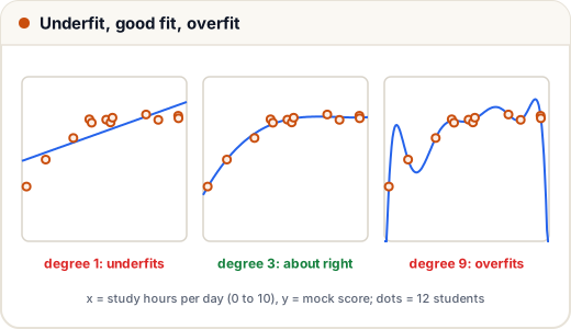
- Degree 1 underfits. A straight line cannot bend, so it is wrong on both training and new data. This error from a too-simple model is called bias.
- Degree 9 overfits. It almost passes through every training point (train MSE 0.2) but is terrible on new students (validation MSE 173). It learned the noise. This sensitivity to the exact training sample is called variance.
- Degree 3 is about right: low error on both.
This is the bias–variance trade-off: more flexible models reduce bias but increase variance. Notice the last column too. The overfitted model needs huge weights to make its sharp swings.
2. The idea: make large weights expensive
Regularisation adds a penalty to the loss:
- Ridge (L2): loss = MSE + λ × (sum of squared weights)
- Lasso (L1): loss = MSE + λ × (sum of absolute weights)
λ (lambda, called alpha in scikit-learn) is the penalty strength. λ = 0 is ordinary regression. A larger λ forces weights towards zero, so the model becomes smoother and less flexible. The bias b is normally not penalised.
For Ridge there is a direct formula: w = (XᵀX + λI)⁻¹ Xᵀy, where I is the identity matrix. That is the lam * np.eye(...) term in fit() above, so we can try it straight away.
3. Ridge rescues the degree-9 model
import numpy as np

rng = np.random.default_rng(1)
def true_score(h):
    return 40 + 8 * h - 0.6 * h ** 2

hours = np.sort(rng.uniform(0, 10, 12))
score = true_score(hours) + rng.normal(0, 3, 12)
val_hours = np.linspace(0, 10, 50)
val_score = true_score(val_hours) + rng.normal(0, 3, 50)

def features(h, degree):
    z = (h - 5) / 3
    return np.column_stack([z ** k for k in range(1, degree + 1)])

def fit(X, y, lam=0.0):
    Xm, ym = X.mean(axis=0), y.mean()
    Xc = X - Xm
    w = np.linalg.solve(Xc.T @ Xc + lam * np.eye(X.shape[1]), Xc.T @ (y - ym))
    return w, ym - Xm @ w

print("lambda  train MSE  validation MSE  largest |weight|")
for lam in (0, 0.1, 1, 10, 100):
    w, b = fit(features(hours, 9), score, lam)
    train = np.mean((features(hours, 9) @ w + b - score) ** 2)
    val = np.mean((features(val_hours, 9) @ w + b - val_score) ** 2)
    print(f"{lam:6}  {train:9.1f}  {val:14.1f}  {np.abs(w).max():12.1f}")
lambda  train MSE  validation MSE  largest |weight|
     0        0.2           173.2          89.0
   0.1        0.8            15.1           4.0
     1        1.5            11.8           2.4
    10        4.6            12.5           0.9
   100       11.3            22.7           0.2
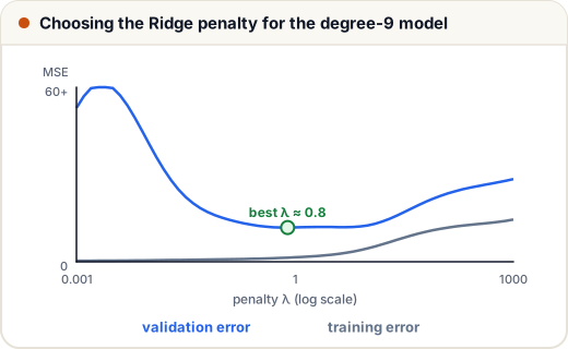
Read the table from top to bottom:
- λ = 0: the overfitted model, weights up to 89.
- λ = 1: weights shrink to at most 2.4 and validation error drops from 173 to about 12. Same 9 features, far better model.
- λ = 100: too much penalty. The weights are squashed almost to zero, the curve becomes nearly flat, and the model underfits again.
Training error always rises as λ grows, because the penalty stops the model from chasing the training points. Validation error falls and then rises. You pick the λ at the bottom of that U, using validation data or cross-validation, never the test set. The test set is kept for one final, honest check.
4. Lasso: shrinking some weights all the way to zero
Lasso's absolute-value penalty has a special effect: it sets unhelpful weights to exactly zero. That makes it an automatic feature selector.
Below, a placement package (in LPA, simulated) truly depends on CGPA, aptitude and coding scores only. We also add three useless columns. Lasso is fitted with coordinate descent: update one weight at a time, and use "soft thresholding" to shrink it by α, stopping at zero.
import numpy as np

rng = np.random.default_rng(5)
n = 60
names = ["cgpa", "aptitude", "coding", "height_cm", "roll_no_digit", "hostel_floor"]
X = np.column_stack([rng.uniform(6, 10, n), rng.uniform(30, 100, n), rng.uniform(0, 100, n),
                     rng.uniform(150, 190, n), rng.integers(0, 10, n), rng.integers(0, 5, n)]).astype(float)
package = 2 + 0.5 * X[:, 0] + 0.03 * X[:, 1] + 0.04 * X[:, 2] + rng.normal(0, 0.5, n)

Z = (X - X.mean(axis=0)) / X.std(axis=0)      # Lasso needs scaled features
y = package - package.mean()

def lasso(Z, y, alpha, rounds=200):
    w = np.zeros(Z.shape[1])
    for _ in range(rounds):
        for j in range(Z.shape[1]):
            residual = y - Z @ w + Z[:, j] * w[j]      # error ignoring feature j
            rho = np.mean(Z[:, j] * residual)
            w[j] = np.sign(rho) * max(abs(rho) - alpha, 0.0)   # soft thresholding
    return w

plain = np.linalg.lstsq(Z, y, rcond=None)[0]
print(f"{'feature':>14}  plain  alpha=0.1  alpha=0.3")
w1, w3 = lasso(Z, y, 0.1), lasso(Z, y, 0.3)
for i, name in enumerate(names):
    print(f"{name:>14}  {plain[i]:5.2f}  {w1[i] + 0:9.2f}  {w3[i] + 0:9.2f}")
       feature  plain  alpha=0.1  alpha=0.3
          cgpa   0.65       0.51       0.27
      aptitude   0.65       0.53       0.34
        coding   1.05       0.92       0.69
     height_cm   0.12       0.00       0.00
 roll_no_digit  -0.02       0.00       0.00
  hostel_floor  -0.03       0.00       0.00
Ordinary regression gives every column some weight, even roll numbers and hostel floors, because it fits small accidental patterns in the noise. With α = 0.1, Lasso sets all three useless features to exactly 0 and keeps the three real ones. With α = 0.3 the real weights shrink too: too strong a penalty starts to hurt.
5. Which one to use?
| Method | Penalty | Effect on weights | Use when |
|---|---|---|---|
| Ridge (L2) | λ × Σw² | shrinks all weights smoothly, rarely to zero | many useful, related features |
| Lasso (L1) | λ × Σ|w| | sets some weights exactly to zero | you suspect many features are useless; want a simpler model |
| Elastic Net | a mix of both | some zeros, stable with related features | many correlated features |
In scikit-learn these are Ridge(alpha=…), Lasso(alpha=…) and ElasticNet(alpha=…, l1_ratio=…). LogisticRegression is regularised by default with an L2 penalty, controlled by C, which is the inverse of the strength: a smaller C means a stronger penalty. Neural networks use the same idea under the name weight decay.
Common mistakes
- Regularising without scaling features. The penalty treats all weights alike, so a feature measured in large units gets a tiny weight and is barely penalised, while others are punished heavily.
- Choosing λ (or α) by looking at the test set. Use validation data or cross-validation.
- Thinking a bigger penalty is always safer. Too much penalty causes underfitting.
- Confusing scikit-learn's
C(bigger = weaker penalty) withalpha(bigger = stronger penalty). - Using Lasso's zero weights as proof that a feature "has no effect". With correlated features Lasso may keep one and drop the other almost at random.
Quick recap
- Underfitting = high bias (too simple); overfitting = high variance (too flexible, learns noise).
- Regularisation adds a penalty on weight size: Ridge uses squares (L2), Lasso uses absolute values (L1).
- Larger λ → smaller weights → smoother model; too large → underfitting.
- Lasso sets useless weights to exactly zero, so it also selects features.
- Choose λ with validation data or cross-validation, and always scale features first.