Python for Data Science & Machine Learning · Lesson 8 of 12 · Updated ·
Machine Learning Basics with scikit-learn — Train/Test Split and Linear Regression
Machine learning means letting a program find patterns in examples instead of writing every rule yourself. Show it thousands of past students (CGPA, internships, projects…) and their packages, and it learns a formula to estimate the package of a new student.
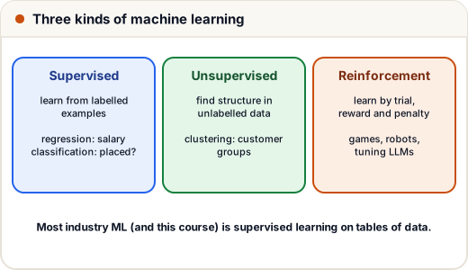
1. Words you must know
| Term | Meaning | Example |
|---|---|---|
| Features (X) | the inputs | CGPA, internships, projects, aptitude |
| Target (y) | what we predict | package in LPA |
| Regression | predict a number | package, house price |
| Classification | predict a category | placed / not placed |
| Training | the model learns from examples | model.fit(X, y) |
| Prediction | apply it to new data | model.predict(X_new) |
2. The workflow
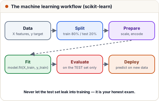
The test set is a final exam the model has never seen. Scoring a model on its own training data is like a student grading their own homework.
3. Practice data
Throughout the ML lessons we use a simulated dataset of 400 students (made with a fixed random seed, so you get the same numbers):
import numpy as np
import pandas as pd

rng = np.random.default_rng(7)
n = 400
df = pd.DataFrame({
    "cgpa": rng.normal(7.5, 0.9, n).clip(5, 10).round(2),
    "internships": rng.integers(0, 3, n),
    "projects": rng.integers(0, 5, n),
    "aptitude": rng.normal(65, 12, n).clip(20, 100).round(),
})
df["package_lpa"] = (3 + 0.9 * (df["cgpa"] - 6) + 0.6 * df["internships"] + 0.25 * df["projects"]
                     + 0.03 * (df["aptitude"] - 50) + rng.normal(0, 0.6, n)).round(2)
print(df.head())
print(df.describe().round(2).loc[["mean", "min", "max"]])
   cgpa  internships  projects  aptitude  package_lpa
0  7.50            1         4      63.0         6.04
1  7.77            2         2      47.0         6.76
2  7.25            0         2      56.0         5.51
3  6.70            0         4      54.0         5.43
4  7.09            1         0      50.0         5.41
      cgpa  internships  projects  aptitude  package_lpa
mean  7.41         0.99      2.04     64.55         5.85
min   5.00         0.00      0.00     36.00         2.07
max   9.53         2.00      4.00     96.00         9.77
4. Train, predict, evaluate
import numpy as np
import pandas as pd
from sklearn.linear_model import LinearRegression
from sklearn.metrics import mean_absolute_error, r2_score
from sklearn.model_selection import train_test_split

rng = np.random.default_rng(7)
n = 400
df = pd.DataFrame({
    "cgpa": rng.normal(7.5, 0.9, n).clip(5, 10).round(2),
    "internships": rng.integers(0, 3, n),
    "projects": rng.integers(0, 5, n),
    "aptitude": rng.normal(65, 12, n).clip(20, 100).round(),
})
df["package_lpa"] = (3 + 0.9 * (df["cgpa"] - 6) + 0.6 * df["internships"] + 0.25 * df["projects"]
                     + 0.03 * (df["aptitude"] - 50) + rng.normal(0, 0.6, n)).round(2)

X = df[["cgpa", "internships", "projects", "aptitude"]]
y = df["package_lpa"]
X_train, X_test, y_train, y_test = train_test_split(X, y, test_size=0.2, random_state=42)

model = LinearRegression()
model.fit(X_train, y_train)                 # learn from the training set only
pred = model.predict(X_test)                # predict the unseen test set

print("MAE (LPA):", round(mean_absolute_error(y_test, pred), 3))
print("R2:", round(r2_score(y_test, pred), 3))
for name, coef in zip(X.columns, model.coef_):
    print(f"{name:12s} {coef:+.3f}")

new_student = pd.DataFrame([{"cgpa": 8.5, "internships": 2, "projects": 3, "aptitude": 75}])
print("predicted package:", model.predict(new_student).round(2)[0], "LPA")
MAE (LPA): 0.476
R2: 0.688
cgpa         +0.872
internships  +0.528
projects     +0.249
aptitude     +0.033
predicted package: 7.93 LPA
Reading the results:
- MAE (mean absolute error): on average the prediction is off by about this many LPA.
- R² (0 to 1): the share of the variation in packages the model explains. 1 is perfect; 0 is no better than always guessing the average.
- Coefficients: each extra internship adds about +0.53 LPA holding the other features fixed. The learned values (0.87, 0.53, 0.25, 0.033) are close to the rules we used to simulate the data (0.9, 0.6, 0.25, 0.03) — not exact, because of the random noise and only 320 training rows. With real data you never know the true rules, which is why the test set matters.
5. Seeing the fit
import numpy as np
import pandas as pd
import matplotlib.pyplot as plt
from sklearn.linear_model import LinearRegression
from sklearn.model_selection import train_test_split

rng = np.random.default_rng(7)
n = 400
df = pd.DataFrame({
    "cgpa": rng.normal(7.5, 0.9, n).clip(5, 10).round(2),
    "internships": rng.integers(0, 3, n),
    "projects": rng.integers(0, 5, n),
    "aptitude": rng.normal(65, 12, n).clip(20, 100).round(),
})
df["package_lpa"] = (3 + 0.9 * (df["cgpa"] - 6) + 0.6 * df["internships"] + 0.25 * df["projects"]
                     + 0.03 * (df["aptitude"] - 50) + rng.normal(0, 0.6, n)).round(2)
X, y = df[["cgpa", "internships", "projects", "aptitude"]], df["package_lpa"]
X_train, X_test, y_train, y_test = train_test_split(X, y, test_size=0.2, random_state=42)
pred = LinearRegression().fit(X_train, y_train).predict(X_test)

fig, ax = plt.subplots(figsize=(5.5, 4.2))
ax.scatter(y_test, pred, alpha=0.7)
lims = [y.min(), y.max()]
ax.plot(lims, lims, color="#c94f0f", label="perfect prediction")
ax.set_xlabel("Actual package (LPA)")
ax.set_ylabel("Predicted package (LPA)")
ax.set_title("Test set: predictions vs reality")
ax.legend()
plt.savefig("regression-fit.svg")
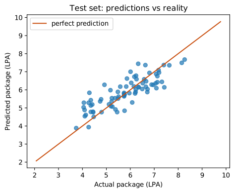
Points close to the diagonal are good predictions; the spread around it is the error the MAE measures.
Common mistakes
- Evaluating on the training data (always looks great, tells you nothing).
- Treating coefficients as causes — with real data they show associations.
- Predicting far outside the training range (a CGPA of 15).
- Forgetting
random_state, so results change every run.
Quick recap
- Supervised learning: features X → target y; regression predicts numbers.
train_test_split,fiton train,predictand score on test.- MAE = typical error in the target's units; R² = share of variation explained.
- Coefficients show each feature's effect, other features held fixed.