Python for Data Science & Machine Learning · Lesson 6 of 12 · Updated ·
Data Visualisation with matplotlib — Bar, Line, Histogram, Scatter and Telling a Story
A good chart answers a question in five seconds. Every chart on this page was drawn by the exact code above it.
1. Which chart?
| Question | Chart |
|---|---|
| Compare categories (branches, cities) | bar |
| Change over time | line |
| How values are spread | histogram (or box plot) |
| Relationship between two numbers | scatter |
| Parts of a whole | stacked bar (pie charts only for 2–3 parts) |
2. Bar chart: compare categories
import matplotlib.pyplot as plt

branches = ["CSE", "IT", "ECE", "ME", "Civil"]
rate = [92, 88, 74, 61, 48]                       # placement rate %

fig, ax = plt.subplots(figsize=(7, 3.6))
bars = ax.bar(branches, rate, color=["#c94f0f" if r == max(rate) else "#94a3b8" for r in rate])
ax.bar_label(bars, fmt="%d%%")                     # value on each bar
ax.set_title("Placement rate by branch, 2026 batch (practice data)")
ax.set_ylabel("Placed (%)")
ax.set_ylim(0, 100)
ax.spines[["top", "right"]].set_visible(False)     # less clutter
plt.savefig("placement-bar.svg")
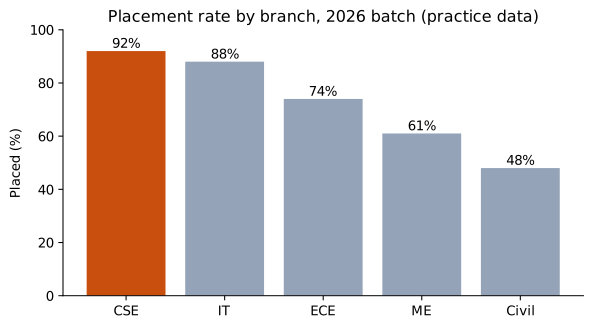
Highlight the one bar that matters, label values directly, remove chart junk.
3. Line chart: trends over time
import matplotlib.pyplot as plt

months = ["Jan", "Feb", "Mar", "Apr", "May", "Jun"]
signups = [120, 135, 160, 210, 340, 310]
paid = [12, 15, 18, 25, 44, 41]

fig, ax = plt.subplots(figsize=(7, 3.6))
ax.plot(months, signups, marker="o", label="Sign-ups")
ax.plot(months, paid, marker="o", label="Paid")
ax.annotate("Exam season", xy=(4, 340), xytext=(1.6, 300), arrowprops={"arrowstyle": "->"})
ax.set_title("Monthly sign-ups (practice data)")
ax.legend()
ax.spines[["top", "right"]].set_visible(False)
plt.savefig("signups-line.svg")
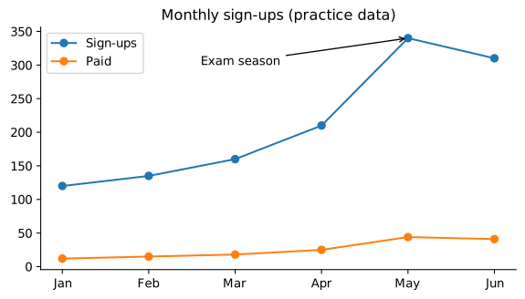
An annotation tells the reader why the line moves — that's the story.
4. Histogram: how values are spread
import numpy as np
import matplotlib.pyplot as plt

rng = np.random.default_rng(1)
cgpa = rng.normal(7.4, 0.8, 500).clip(4, 10)

fig, ax = plt.subplots(figsize=(7, 3.6))
ax.hist(cgpa, bins=20, color="#2563eb", edgecolor="white")
ax.axvline(cgpa.mean(), color="#c94f0f", linestyle="--", label=f"mean {cgpa.mean():.2f}")
ax.set_title("CGPA of 500 students (simulated)")
ax.set_xlabel("CGPA")
ax.set_ylabel("Students")
ax.legend()
plt.savefig("cgpa-hist.svg")
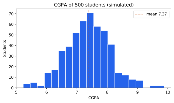
5. Scatter plot: relationships
import numpy as np
import matplotlib.pyplot as plt

rng = np.random.default_rng(3)
cgpa = rng.uniform(6, 10, 120)
package = 2 + 1.1 * (cgpa - 6) + rng.normal(0, 0.8, 120)

fig, ax = plt.subplots(figsize=(7, 3.6))
ax.scatter(cgpa, package, alpha=0.6)
slope, intercept = np.polyfit(cgpa, package, 1)        # best-fit straight line
xs = np.array([6, 10])
ax.plot(xs, slope * xs + intercept, color="#c94f0f", label=f"trend: +{slope:.2f} LPA per CGPA point")
ax.set_xlabel("CGPA")
ax.set_ylabel("Package (LPA)")
ax.set_title("Higher CGPA, higher package — on average (simulated)")
ax.legend()
plt.savefig("cgpa-package-scatter.svg")
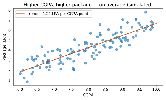
Remember: a trend is not a guarantee for each person, and correlation is not causation (lesson 7).
6. Several charts together
import numpy as np
import matplotlib.pyplot as plt

rng = np.random.default_rng(5)
aptitude = rng.normal(62, 12, 300).clip(0, 100)

fig, (left, right) = plt.subplots(1, 2, figsize=(8, 3.4))
left.hist(aptitude, bins=15, color="#7c3aed", edgecolor="white")
left.set_title("Aptitude scores")
right.boxplot(aptitude, orientation="horizontal")
right.set_title("Same data as a box plot")
fig.tight_layout()
plt.savefig("aptitude-subplots.svg")
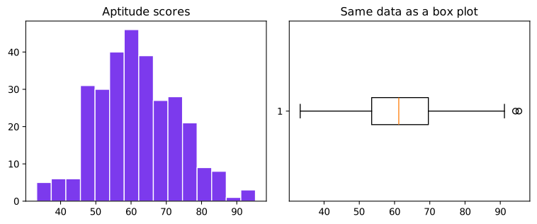
The box plot shows median, middle 50% (the box) and outliers (dots) — compact for comparing many groups.
Chart rules that impress managers
- A title that states the finding, not just the topic.
- Label axes with units; label values directly where possible.
- One highlight colour; everything else grey.
- Start bar charts at zero.
- Say where the data comes from and whether it's a sample.
(For interactive dashboards look at Plotly, Power BI or Tableau; seaborn gives prettier statistical charts with less code.)
Common mistakes
- Pie charts with 8 slices; 3-D charts.
- Bar charts not starting at zero (exaggerates differences).
- Rainbow colours with no meaning.
- No title or units.
Quick recap
- Bar → compare, line → trend, histogram/box → spread, scatter → relationship.
fig, ax = plt.subplots(), thenax.bar / plot / hist / scatter, labels,savefig.- Highlight, annotate, simplify.