Unsupervised Learning — K-Means Clustering, the Elbow Method and PCA

Supervised learning needs labels. Often you have none — just behaviour data — and the question is "what kinds of users do we have?" That's unsupervised learning.

Case study: segmenting learners

An online learning platform wants to send different messages to different kinds of learners. For each learner it knows hours studied per week and quizzes taken per week. No labels exist — we let the data suggest the groups.

1. K-means in four steps

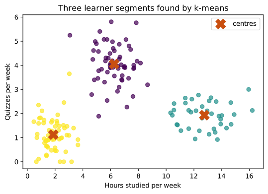
K-means picks k centres, assigns each point to its nearest centre, moves each centre to the middle of its points, and repeats until nothing changes.

import numpy as np
import matplotlib.pyplot as plt
from sklearn.cluster import KMeans

rng = np.random.default_rng(4)
casual = rng.normal([2, 1], [0.8, 0.6], (60, 2))       # practice data with three hidden groups
steady = rng.normal([6, 4], [1.0, 0.8], (60, 2))
crammers = rng.normal([12, 2], [1.5, 0.7], (40, 2))
X = np.vstack([casual, steady, crammers]).clip(0)

km = KMeans(n_clusters=3, n_init=10, random_state=0).fit(X)

fig, ax = plt.subplots(figsize=(6.5, 4.2))
ax.scatter(X[:, 0], X[:, 1], c=km.labels_, cmap="viridis", alpha=0.7)
ax.scatter(km.cluster_centers_[:, 0], km.cluster_centers_[:, 1], marker="X", s=220, c="#c94f0f", label="centres")
ax.set_xlabel("Hours studied per week")
ax.set_ylabel("Quizzes per week")
ax.set_title("Three learner segments found by k-means")
ax.legend()
plt.savefig("kmeans-segments.svg")

2. Choosing k: the elbow method

import numpy as np
import matplotlib.pyplot as plt
from sklearn.cluster import KMeans

rng = np.random.default_rng(4)
X = np.vstack([rng.normal([2, 1], [0.8, 0.6], (60, 2)),
               rng.normal([6, 4], [1.0, 0.8], (60, 2)),
               rng.normal([12, 2], [1.5, 0.7], (40, 2))]).clip(0)

ks = range(1, 9)
inertia = [KMeans(n_clusters=k, n_init=10, random_state=0).fit(X).inertia_ for k in ks]

fig, ax = plt.subplots(figsize=(6.5, 3.6))
ax.plot(ks, inertia, marker="o")
ax.set_xlabel("k (number of clusters)")
ax.set_ylabel("Inertia (within-cluster spread)")
ax.set_title("The 'elbow' at k = 3: more clusters barely help after that")
plt.savefig("kmeans-elbow.svg")

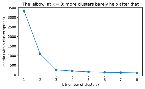
Inertia always falls as k grows; pick the k where the improvement suddenly slows (the elbow). Also ask: can the business act on that many segments?

3. Describing the segments

Clusters are only useful when people can understand them:

import numpy as np
import pandas as pd
from sklearn.cluster import KMeans

rng = np.random.default_rng(4)
X = np.vstack([rng.normal([2, 1], [0.8, 0.6], (60, 2)),
               rng.normal([6, 4], [1.0, 0.8], (60, 2)),
               rng.normal([12, 2], [1.5, 0.7], (40, 2))]).clip(0)
df = pd.DataFrame(X, columns=["hours", "quizzes"])
df["segment"] = KMeans(n_clusters=3, n_init=10, random_state=0).fit_predict(X)

profile = df.groupby("segment").agg(learners=("hours", "size"), hours=("hours", "mean"), quizzes=("quizzes", "mean")).round(1)
print(profile.sort_values("hours"))

         learners  hours  quizzes
segment                          
2              61    1.9      1.1
0              60    6.3      4.1
1              39   12.8      1.9

Now name them: casual (few hours, few quizzes → send short daily questions), steady (moderate hours, lots of quizzes → offer certificates and contests), crammers (many hours, few quizzes → nudge them to test themselves, not just read). The cluster numbers themselves mean nothing — the profile does.

4. Scale before clustering

K-means uses distances. If one feature is in rupees (0–50,000) and another in hours (0–20), rupees dominate everything. Scale features first (StandardScaler), as in the previous lesson.

5. PCA: many features → two

Principal Component Analysis finds new axes that keep as much variation as possible, so data with many features can be plotted in 2-D or compressed:

import numpy as np
from sklearn.decomposition import PCA
from sklearn.preprocessing import StandardScaler

rng = np.random.default_rng(9)
base = rng.normal(size=(300, 2))
# six measured features that are really driven by two underlying factors (+ noise)
features = np.column_stack([base[:, 0], base[:, 0] * 0.9, base[:, 0] * -0.7,
                            base[:, 1], base[:, 1] * 1.1, base[:, 0] + base[:, 1]])
features += rng.normal(0, 0.2, features.shape)

pca = PCA(n_components=6).fit(StandardScaler().fit_transform(features))
print("variance explained by each component:", pca.explained_variance_ratio_.round(3))
print("first two together:", pca.explained_variance_ratio_[:2].sum().round(3))

variance explained by each component: [0.567 0.403 0.012 0.007 0.006 0.004]
first two together: 0.971

Six measurements, but two components keep almost all the information — because the data really had two underlying factors. PCA is used for visualisation, speeding up models, and removing redundant features.

Common mistakes

• Forgetting to scale before k-means or PCA.
• Treating cluster numbers (0, 1, 2) as meaningful labels.
• Choosing k by the elbow alone, ignoring whether the business can use the segments.
• Using k-means on data with odd-shaped groups (look at DBSCAN or hierarchical clustering then).

Quick recap

• Unsupervised learning finds structure without labels.
• K-means: choose k (elbow + business sense), scale features, profile and name clusters.
• PCA compresses correlated features into a few components that keep most variation.