Statistics for Data Science — Averages, Spread, Distributions, Correlation and A/B Tests

You don't need a statistics degree for data work — but you do need these ideas to avoid embarrassing (and expensive) wrong conclusions.

1. Mean vs median: the salary trap

import numpy as np

packages = np.array([3.5, 3.6, 3.6, 4.0, 4.2, 4.5, 5.0, 6.0, 7.5, 45.0])   # LPA, one star offer
print("mean  ", packages.mean().round(2))
print("median", np.median(packages))
print("mean without the 45 LPA offer", packages[:-1].mean().round(2))

mean   8.69
median 4.35
mean without the 45 LPA offer 4.66

One 45 LPA offer pulls the mean up a lot; the median barely moves. When a coaching ad says "average package 8.69 LPA", ask for the median (here 4.35) — most students got far less. Use the median for skewed data (salaries, house prices, delivery times).

2. Spread: standard deviation and percentiles

import numpy as np

batch_a = np.array([68, 70, 71, 72, 69, 70, 71])
batch_b = np.array([40, 95, 60, 88, 52, 79, 76])
print("means:", batch_a.mean().round(1), batch_b.mean().round(1))
print("std:  ", batch_a.std().round(1), batch_b.std().round(1))
print("90th percentile of B:", np.percentile(batch_b, 90).round(1))

means: 70.1 70.0
std:   1.2 18.5
90th percentile of B: 90.8

Same average, completely different batches: standard deviation measures how spread out values are. A percentile says "90% of values are below this" — that's how exam ranks like "98 percentile" work.

3. The normal distribution

Many measurements (heights, exam marks, measurement errors) form a bell curve. For a normal distribution about 68% of values lie within 1 standard deviation of the mean, 95% within 2, and 99.7% within 3:

import numpy as np

rng = np.random.default_rng(0)
marks = rng.normal(loc=60, scale=10, size=100_000)
for k in (1, 2, 3):
    inside = np.mean(np.abs(marks - 60) <= k * 10) * 100
    print(f"within {k} sd: {inside:.1f}%")

within 1 sd: 68.4%
within 2 sd: 95.5%
within 3 sd: 99.7%

import numpy as np
import matplotlib.pyplot as plt

x = np.linspace(20, 100, 400)
pdf = np.exp(-((x - 60) ** 2) / (2 * 10 ** 2)) / (10 * np.sqrt(2 * np.pi))

fig, ax = plt.subplots(figsize=(7, 3.4))
ax.plot(x, pdf, color="#0f1626")
for k, colour in ((3, "#dbeafe"), (2, "#93c5fd"), (1, "#2563eb")):
    band = (x >= 60 - k * 10) & (x <= 60 + k * 10)
    ax.fill_between(x[band], pdf[band], color=colour)
ax.set_title("Marks ~ normal(mean 60, sd 10): 68% within 50–70, 95% within 40–80")
ax.set_xlabel("Marks")
ax.set_yticks([])
ax.spines[["top", "right", "left"]].set_visible(False)
plt.savefig("normal-68-95.svg")

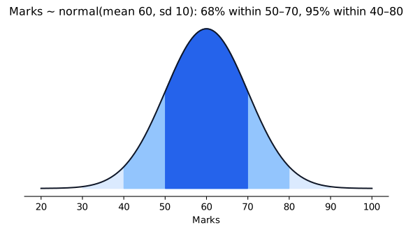
The simulation confirms the 68–95–99.7 rule. A z-score (x − mean) / sd tells how unusual a value is: z = 2.5 is rare.

4. Correlation is not causation

import numpy as np

rng = np.random.default_rng(2)
study_hours = rng.uniform(0, 6, 200)
marks = 40 + 8 * study_hours + rng.normal(0, 8, 200)
phone_hours = 8 - study_hours + rng.normal(0, 1, 200)
print("study vs marks:", np.corrcoef(study_hours, marks)[0, 1].round(2))
print("phone vs marks:", np.corrcoef(phone_hours, marks)[0, 1].round(2))

study vs marks: 0.85
phone vs marks: -0.74

Correlation runs from −1 (perfect opposite) through 0 (none) to +1 (perfect together). Here phone time is strongly negatively correlated with marks — but in our simulation phone time doesn't affect marks at all; both are driven by study hours (a confounder). Only a controlled experiment can show cause.

5. A/B testing: did the change work?

Case: an ed-tech app tests a new "Start free trial" button. Version A (old) and B (new) are each shown to 2,000 random visitors.

import numpy as np

rng = np.random.default_rng(11)
a = rng.random(2000) < 0.050          # old button: true rate 5.0%
b = rng.random(2000) < 0.065          # new button: true rate 6.5%
print(f"A: {a.mean():.2%}  B: {b.mean():.2%}")

# Permutation test: if the button made no difference, how often would random shuffling
# produce a gap at least this big?
observed = b.mean() - a.mean()
both = np.concatenate([a, b])
gaps = []
for _ in range(5000):
    rng.shuffle(both)
    gaps.append(both[2000:].mean() - both[:2000].mean())
p_value = np.mean(np.array(gaps) >= observed)
print(f"observed gap {observed:.2%}, p-value {p_value:.3f}")

A: 5.10%  B: 6.00%
observed gap 0.90%, p-value 0.116

The p-value is the chance of seeing a gap this large if the button changed nothing. Below 0.05 we usually call the result statistically significant.

Look closely at this run: we built B to be better (6.5% vs 5.0%), yet with 2,000 visitors each the observed gap is only 0.9 points and the p-value is about 0.12 — not significant. The data can't yet rule out luck. That's the real lesson of A/B testing: small true improvements need large samples. Decide the sample size before the test (from the smallest gain worth detecting), never stop early because the result "looks good", and also ask whether the gain is big enough to matter for the business.

Common mistakes

• Reporting the mean for skewed data.
• Saying "X causes Y" from a correlation.
• Small samples: 30 users can't settle an A/B test.
• Running many tests and reporting only the one with p < 0.05.

Quick recap

• Median for skewed data; standard deviation and percentiles for spread.
• Normal distribution: 68–95–99.7 rule; z-scores measure unusualness.
• Correlation (−1 to +1) ≠ causation; watch for confounders.
• A/B tests: random split, fixed sample size, p-value < 0.05 plus a meaningful effect.