AdvancedPython for Data Science & Machine Learning · Lesson 17 of 21 · Updated ·
Time Series with pandas — Dates, Resampling, Rolling Averages, Lags and Simple Forecasts
Sales per day, sign-ups per hour, app crashes per minute, a city's temperature: whenever rows are ordered in time, the order itself carries information. Yesterday tells you something about today; last Monday tells you something about this Monday. This lesson covers the pandas tools for such time series and the forecasting baselines every analyst should try first.
1. A series with a date index
Case: an ed-tech platform records daily sign-ups for a placement course. The manager asks: Are sign-ups growing? Which days are busy? How many should we expect next week?
import numpy as np
import pandas as pd

rng = np.random.default_rng(5)
days = pd.date_range("2026-03-02", periods=56, freq="D")          # 8 weeks, starting on a Monday
weekday_effect = np.array([10, 8, 6, 4, 0, -12, -16])             # Mon ... Sun (practice data)
signups = 60 + 0.5 * np.arange(56) + weekday_effect[days.dayofweek] + rng.normal(0, 4, 56)
s = pd.Series(signups.round().astype("int64"), index=days, name="signups")

print(s.head(8))
print("from", s.index.min().date(), "to", s.index.max().date(), "| total", s.sum())
2026-03-02    67
2026-03-03    63
2026-03-04    66
2026-03-05    67
2026-03-06    67
2026-03-07    51
2026-03-08    45
2026-03-09    70
Freq: D, Name: signups, dtype: int64
from 2026-03-02 to 2026-04-26 | total 4062
With a DatetimeIndex you can select by date strings (s["2026-03-09":"2026-03-15"]), and pandas understands weeks, months and weekdays.
2. Resampling: change the time unit
resample is groupby for time: it puts rows into time buckets and aggregates each bucket.
import numpy as np
import pandas as pd

rng = np.random.default_rng(5)
days = pd.date_range("2026-03-02", periods=56, freq="D")
weekday_effect = np.array([10, 8, 6, 4, 0, -12, -16])
s = pd.Series((60 + 0.5 * np.arange(56) + weekday_effect[days.dayofweek] + rng.normal(0, 4, 56)).round().astype("int64"), index=days)

weekly = s.resample("W").sum()           # weeks ending on Sunday
print(weekly)
print("week-on-week change (%):", weekly.pct_change().mul(100).round(1).tolist()[1:])
2026-03-08    426
2026-03-15    460
2026-03-22    462
2026-03-29    501
2026-04-05    514
2026-04-12    546
2026-04-19    559
2026-04-26    594
Freq: W-SUN, dtype: int64
week-on-week change (%): [8.0, 0.4, 8.4, 2.6, 6.2, 2.4, 6.3]
Daily numbers jump around; weekly totals show the trend clearly. Other common frequencies: "h" (hour), "D" (day), "MS" (month start), "ME" (month end), "QE" (quarter end).
3. Rolling averages and weekday patterns
A rolling (moving) average smooths the noise: each point becomes the mean of the last n points.
import numpy as np
import pandas as pd

rng = np.random.default_rng(5)
days = pd.date_range("2026-03-02", periods=56, freq="D")
weekday_effect = np.array([10, 8, 6, 4, 0, -12, -16])
s = pd.Series((60 + 0.5 * np.arange(56) + weekday_effect[days.dayofweek] + rng.normal(0, 4, 56)).round().astype("int64"), index=days)

rolling = s.rolling(7).mean()            # first 6 values are NaN: not enough history yet
print(rolling.dropna().round(1).iloc[[0, 14, 28, 49]])

by_day = s.groupby(s.index.day_name()).mean().round(1)
print(by_day.reindex(["Monday", "Tuesday", "Wednesday", "Thursday", "Friday", "Saturday", "Sunday"]))
2026-03-08    60.9
2026-03-22    66.0
2026-04-05    73.4
2026-04-26    84.9
dtype: float64
Monday       80.0
Tuesday      79.8
Wednesday    77.2
Thursday     78.4
Friday       73.2
Saturday     60.6
Sunday       58.5
dtype: float64
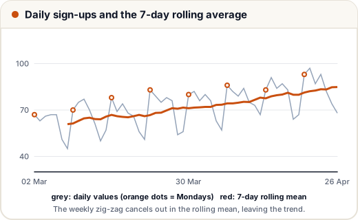
A 7-day window is the natural choice here because the pattern repeats every week (weekly seasonality): every window contains exactly one Monday and one Sunday, so the weekday ups and downs cancel out and only the trend remains. The weekday table shows the pattern itself: Mondays are busy, weekends are quiet — useful for planning when to send promotional emails or schedule support staff.
4. Lags and changes: features from the past
To predict today, a model can use lag features — values from earlier days. shift(k) moves the series down by k steps:
import pandas as pd

s = pd.Series([50, 54, 61, 58, 70], index=pd.date_range("2026-04-01", periods=5, freq="D"))
df = pd.DataFrame({
    "signups": s,
    "yesterday": s.shift(1),
    "change": s.diff(),                     # today - yesterday
    "pct_change": s.pct_change().mul(100).round(1),
})
print(df)
            signups  yesterday  change  pct_change
2026-04-01       50        NaN     NaN         NaN
2026-04-02       54       50.0     4.0         8.0
2026-04-03       61       54.0     7.0        13.0
2026-04-04       58       61.0    -3.0        -4.9
2026-04-05       70       58.0    12.0        20.7
| Method | Gives | Typical use |
|---|---|---|
shift(1) | yesterday's value on today's row | lag feature for a model |
shift(7) | same weekday last week | weekly seasonality |
diff() | change from the previous row | growth per day |
pct_change() | relative change | week-on-week growth in % |
rolling(n).mean() | smoothed level | trend, dashboards |
The first row has NaN because there is no "yesterday" for it. Drop such rows before training a model.
5. Baseline forecasts — and how to test them honestly
Before any machine learning, try simple baselines. A fancy model that can't beat them is not worth deploying.
- Naive: tomorrow = today.
- Seasonal naive: tomorrow = the same weekday last week.
- Moving average: tomorrow = mean of the last 7 days.
Test them the way they will be used: train on the past, test on the future. Here the last 14 days are the test period:
import numpy as np
import pandas as pd

rng = np.random.default_rng(5)
days = pd.date_range("2026-03-02", periods=56, freq="D")
weekday_effect = np.array([10, 8, 6, 4, 0, -12, -16])
s = pd.Series((60 + 0.5 * np.arange(56) + weekday_effect[days.dayofweek] + rng.normal(0, 4, 56)).round().astype("int64"), index=days)

forecasts = pd.DataFrame({
    "actual": s,
    "naive": s.shift(1),
    "seasonal_naive": s.shift(7),
    "moving_avg_7": s.rolling(7).mean().shift(1),     # shift(1): use only days BEFORE the one we predict
})
test = forecasts.loc["2026-04-13":]                    # the last 14 days
print("test days:", len(test), "| from", test.index[0].date())
for method in ["naive", "seasonal_naive", "moving_avg_7"]:
    mae = (test["actual"] - test[method]).abs().mean()
    print(f"{method:15s} MAE = {mae:.1f} sign-ups")
test days: 14 | from 2026-04-13
naive           MAE = 9.4 sign-ups
seasonal_naive  MAE = 5.3 sign-ups
moving_avg_7    MAE = 9.7 sign-ups
The seasonal naive forecast wins easily, because it is the only one that knows Monday follows Sunday. That's a business insight in itself: the weekday pattern matters more than yesterday's number. A real model (with lag-7 features, a trend and holidays) must now beat this MAE to earn its place.
Notice .shift(1) after the rolling mean. Without it, the moving average for a day would include that same day — the forecast would secretly peek at the answer.
6. Never split time series at random
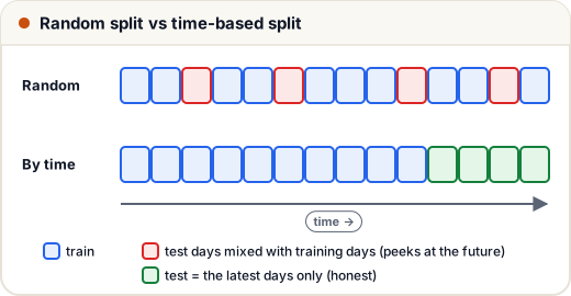
With a random train/test split, the model trains on Wednesday and Friday and is "tested" on the Thursday in between — it effectively sees the future. Scores look brilliant and collapse in production. Always split by date (scikit-learn's TimeSeriesSplit does this for cross-validation), and build every feature only from information available before the moment you predict.
Common mistakes
- Splitting time series randomly, or computing rolling features that include the day being predicted.
- Comparing a model only with nothing, instead of with naive and seasonal-naive baselines.
- Treating dates as text — convert with
pd.to_datetimeand set them as the index. - A rolling window that doesn't match the seasonality (5 days for a weekly pattern).
- Ignoring holidays and special events (exam weeks, festivals, sales) that break the usual pattern.
Quick recap
- Use a
DatetimeIndex;resamplechanges the time unit;rollingsmooths. - Look for trend and seasonality (weekday patterns with
groupby(index.day_name())). shift,diffandpct_changebuild lag and change features.- Always try naive, seasonal-naive and moving-average baselines first.
- Split by time and never let a feature see the future.