AdvancedPython for Data Science & Machine Learning · Lesson 13 of 15 · Updated ·
Probability and Bayes' Theorem for Data Science — Conditional Probability, Base Rates and Naive Bayes
Every classifier, every A/B test and every risk score is built on probability. You don't need heavy formulas — most of what a data scientist uses is counting carefully and asking "out of whom?". This lesson builds that habit, then uses it to write a working spam filter.
1. Probability is counting
The probability of an event is (number of ways it happens) ÷ (number of equally likely cases). With data, it is simply a share of rows.
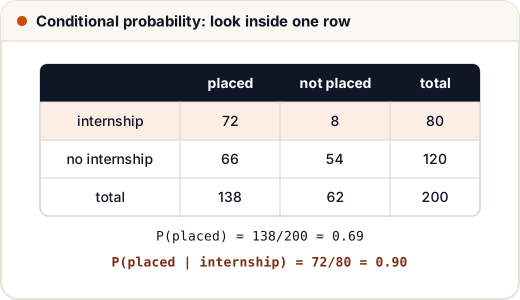
A placement cell has records of 200 final-year students: did they do an internship, and were they placed?
counts = {                                    # 200 final-year students (practice data)
    ("internship", "placed"): 72, ("internship", "not placed"): 8,
    ("no internship", "placed"): 66, ("no internship", "not placed"): 54,
}
total = sum(counts.values())
placed = counts[("internship", "placed")] + counts[("no internship", "placed")]
interned = counts[("internship", "placed")] + counts[("internship", "not placed")]

print("P(placed)                =", placed / total)
print("P(internship)            =", interned / total)
print("P(placed and internship) =", counts[("internship", "placed")] / total)
print("P(placed | internship)   =", counts[("internship", "placed")] / interned)
print("P(placed | no internship)=", round(counts[("no internship", "placed")] / (total - interned), 2))
P(placed)                = 0.69
P(internship)            = 0.4
P(placed and internship) = 0.36
P(placed | internship)   = 0.9
P(placed | no internship)= 0.55
Read P(placed | internship) as "probability of placed given internship". The bar | means: only look at the rows where the condition is true. So the denominator changes from all 200 students to the 80 who did an internship.
2. Conditional probability and independence
The formula behind the code is:
P(A | B) = P(A and B) ÷ P(B)
Check it: 0.36 ÷ 0.4 = 0.9. Same answer as counting inside the row.
Two events are independent when knowing one tells you nothing about the other, that is P(A | B) = P(A). Here P(placed) is 0.69 but P(placed | internship) is 0.9, so placement and internships are not independent — they are associated. (Associated, not "caused by": strong students may simply be more likely to get internships. See the correlation section of the statistics lesson.)
| Rule | Formula | Example |
|---|---|---|
| Complement | P(not A) = 1 − P(A) | P(not placed) = 1 − 0.69 = 0.31 |
| Multiplication | P(A and B) = P(A) × P(B | A) | 0.4 × 0.9 = 0.36 |
| Independent events | P(A and B) = P(A) × P(B) | two fair coin tosses: 0.5 × 0.5 |
| Addition | P(A or B) = P(A) + P(B) − P(A and B) | 0.69 + 0.4 − 0.36 = 0.73 |
A very common mistake is mixing up P(A | B) and P(B | A). "90% of interns got placed" is not the same as "90% of placed students were interns" (that one is 72 ÷ 138 ≈ 0.52).
3. Bayes' theorem: turning a probability around
Bayes' theorem lets you go from P(evidence | cause) — which is usually what you know — to P(cause | evidence) — which is what you want:
P(cause | evidence) = P(evidence | cause) × P(cause) ÷ P(evidence)
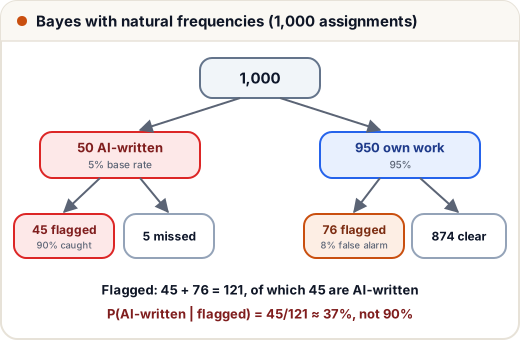
Case: a college runs every assignment through a tool that flags "AI-written" text. Suppose the tool catches 90% of AI-written assignments, but also wrongly flags 8% of honest ones, and about 5% of assignments are really AI-written. A student's work is flagged. How likely is it that the work is really AI-written?
Most people guess "about 90%". Let's count with 1,000 assignments:
def bayes(prior, hit_rate, false_alarm_rate):
    """P(cause | flagged) from P(cause), P(flag | cause) and P(flag | no cause)."""
    p_flag = prior * hit_rate + (1 - prior) * false_alarm_rate      # all ways to be flagged
    return prior * hit_rate / p_flag

print(f"P(AI-written | flagged) = {bayes(0.05, 0.90, 0.08):.3f}")
for prior in (0.01, 0.05, 0.20, 0.50):
    print(f"if {prior:4.0%} of work is AI-written -> {bayes(prior, 0.90, 0.08):.0%} of flags are right")
P(AI-written | flagged) = 0.372
if   1% of work is AI-written -> 10% of flags are right
if   5% of work is AI-written -> 37% of flags are right
if  20% of work is AI-written -> 74% of flags are right
if  50% of work is AI-written -> 92% of flags are right
Only about 37% of flagged assignments are really AI-written. The reason is the base rate (also called the prior): honest work is so common that even a small false-alarm rate on it produces more flags (76) than the real cases do (45). As the base rate rises, the same tool becomes much more trustworthy.
This is the base-rate trap, and it appears everywhere: fraud alerts, medical screening, spam filters, "at-risk student" models. A flag is evidence, not proof — which is why a flagged case should go to a human, not straight to a penalty.
We can check the formula by simulation, as data scientists often do:
import numpy as np

rng = np.random.default_rng(0)
n = 200_000
ai_written = rng.random(n) < 0.05
flagged = np.where(ai_written, rng.random(n) < 0.90, rng.random(n) < 0.08)
print("flagged assignments:", flagged.sum())
print("share of flagged that are AI-written:", round(ai_written[flagged].mean(), 3))
flagged assignments: 24067
share of flagged that are AI-written: 0.368
The simulation gives 0.368, very close to the 0.372 from Bayes' theorem (a simulation always has a little random noise).
4. Naive Bayes: a spam filter from scratch
A Naive Bayes classifier applies Bayes' theorem to text. For each class (spam or genuine) it learns how often each word appears, then for a new message it compares:
score(class) = log P(class) + Σ log P(word | class)
It is "naive" because it assumes words are independent of each other given the class — not true, but the classifier still works surprisingly well, trains in one pass, and is a classic interview topic.
import math
from collections import Counter

train = [
    ("win free recharge now", "spam"), ("free gift claim now", "spam"),
    ("earn money from home click link", "spam"), ("claim your free prize", "spam"),
    ("placement drive on monday", "ok"), ("submit the assignment by friday", "ok"),
    ("aptitude test link for monday", "ok"), ("class moved to room 204", "ok"),
]
word_counts = {"spam": Counter(), "ok": Counter()}
class_counts = Counter()
for text, label in train:
    class_counts[label] += 1
    word_counts[label].update(text.split())
vocab = set(w for c in word_counts.values() for w in c)

def score(text, label):
    s = math.log(class_counts[label] / len(train))              # prior
    total = sum(word_counts[label].values())
    for w in text.split():
        # Laplace smoothing: +1 so an unseen word doesn't make the probability 0
        s += math.log((word_counts[label][w] + 1) / (total + len(vocab)))
    return s

for msg in ["claim free recharge", "test on monday", "free aptitude test link"]:
    scores = {label: score(msg, label) for label in ("spam", "ok")}
    best = max(scores, key=scores.get)
    print(f"{msg!r:28} spam={scores['spam']:.2f} ok={scores['ok']:.2f} -> {best}")
'claim free recharge'        spam=-9.19 ok=-12.43 -> spam
'test on monday'             spam=-12.37 ok=-9.94 -> ok
'free aptitude test link'    spam=-14.18 ok=-14.26 -> spam
Two details matter in every real implementation:
- Logs instead of products. Multiplying many small probabilities underflows to 0.0 on a computer; adding their logs is safe. The larger (less negative) score wins.
- Laplace smoothing. Without the
+ 1, a single word never seen in spam (like "monday") would make P(spam) exactly zero, whatever else the message says.
Look at the last message: "free" pulls it towards spam, while "aptitude", "test" and "link" pull it towards genuine messages. The two scores are almost equal (−14.18 vs −14.26), so it is labelled spam by a hair. With only eight training messages that is expected; a real filter learns from thousands of messages and often has a "not sure" zone where close calls go to the inbox instead of the spam folder.
Common mistakes
- Confusing P(A | B) with P(B | A) ("most placed students were interns" vs "most interns were placed").
- Ignoring the base rate, and trusting a "90% accurate" flag on a rare event.
- Multiplying many probabilities directly instead of adding logs.
- Forgetting smoothing, so one unseen word gives a probability of zero.
- Treating an association (internship ↔ placement) as proof of cause.
Quick recap
- Probability from data = share of rows; P(A | B) means "only among rows where B is true".
- P(A | B) = P(A and B) ÷ P(B); independent events have P(A | B) = P(A).
- Bayes' theorem turns P(evidence | cause) into P(cause | evidence); the prior (base rate) matters a lot.
- Draw a natural-frequency tree (out of 1,000) to avoid the base-rate trap.
- Naive Bayes = prior × word likelihoods, computed with logs and Laplace smoothing.