AdvancedPython for Data Science & Machine Learning · Lesson 15 of 15 · Updated ·
Hypothesis Testing — t-Tests, Paired Tests, Chi-Square, p-Values and Type I/II Errors
The statistics lesson showed one A/B test. Real questions come in a few standard shapes: Do two groups differ? Did the same students improve? Are two categories related? Each shape has a standard hypothesis test. This lesson computes each one by hand (so you understand it), and names the library function you would use at work.
1. The five steps
- Null hypothesis (H₀) — "nothing is going on": no difference, no effect, no relationship.
- Alternative hypothesis (H₁) — what you suspect: there is a difference.
- Significance level (α) — chosen before looking at results; usually 0.05.
- Test statistic and p-value — how surprising the data would be if H₀ were true.
- Decision — if p < α, reject H₀; otherwise you fail to reject it. (Not "prove H₀" — absence of evidence is not evidence of absence.)
2. Two groups: the two-sample t-test
Question: a college offered an optional aptitude coaching course. Did students who took it score higher on the mock placement test?
The t-statistic is the difference in means divided by its standard error — "how many standard errors apart are the two groups?" The version below (Welch's t-test) does not assume both groups have the same spread.
import numpy as np

coached = np.array([68, 74, 71, 80, 77, 69, 83, 75, 72, 78, 81, 70])
not_coached = np.array([65, 70, 62, 73, 68, 66, 71, 64, 69, 67, 74, 63])

def welch_t(a, b):
    se = np.sqrt(a.var(ddof=1) / len(a) + b.var(ddof=1) / len(b))
    return (a.mean() - b.mean()) / se

t_obs = welch_t(coached, not_coached)
print(f"means: {coached.mean():.2f} vs {not_coached.mean():.2f}, t = {t_obs:.2f}")

# p-value by permutation: if coaching made no difference, the labels are arbitrary — shuffle them
rng = np.random.default_rng(0)
both = np.concatenate([coached, not_coached])
count = 0
for _ in range(10_000):
    rng.shuffle(both)
    if abs(welch_t(both[:12], both[12:])) >= abs(t_obs):     # two-sided: a difference in either direction
        count += 1
print("p-value:", count / 10_000)
means: 74.83 vs 67.67, t = 3.93
p-value: 0.0011
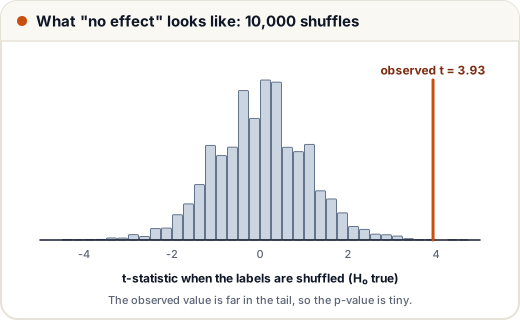
The shuffled t-values show what "no effect" looks like; our observed t is far out in the tail, so the p-value is tiny and we reject H₀. At work you would call scipy.stats.ttest_ind(coached, not_coached, equal_var=False), which gives the same t and a p-value from the t-distribution instead of shuffling.
But be careful with the conclusion. Students chose to take coaching; motivated students may score higher anyway. The test says the groups differ — not that coaching caused it. Only random assignment (an experiment) supports a causal claim.
3. Same students twice: the paired test
Question: ten students took a mock test, did two weeks of practice, then took another. Did they improve?
These are not two independent groups — each "after" score belongs to a "before" score. Analyse the differences:
import numpy as np

before = np.array([52, 61, 47, 70, 58, 66, 49, 55, 63, 60])
after  = np.array([58, 63, 55, 71, 64, 65, 56, 60, 70, 62])
d = after - before
t = d.mean() / (d.std(ddof=1) / np.sqrt(len(d)))
print("differences:", d)
print(f"mean improvement {d.mean():.1f} marks, paired t = {t:.2f}")

# permutation for paired data: under H0 each difference is equally likely to be + or −
rng = np.random.default_rng(1)
signs = rng.choice([-1, 1], size=(10_000, len(d)))
fake = (signs * d).mean(axis=1)
print("p-value:", np.mean(np.abs(fake) >= abs(d.mean())))
differences: [ 6  2  8  1  6 -1  7  5  7  2]
mean improvement 4.3 marks, paired t = 4.45
p-value: 0.0055
Pairing removes the big differences between students (some always score 50, others 70) and keeps only the change within each student. That makes the test far more sensitive. The library function is scipy.stats.ttest_rel(after, before). Treating paired data as two independent groups is a classic mistake.
4. Two categories: the chi-square test
Question: does branch relate to whether students prefer online or offline classes? The data is a table of counts, so means don't apply. The chi-square (χ²) test of independence compares the observed counts with the counts we would expect if the two variables were unrelated:
expected = row total × column total ÷ grand total, and χ² = Σ (observed − expected)² ÷ expected
import numpy as np

observed = np.array([[45, 35],     # CSE: online, offline
                     [25, 35],     # ECE
                     [15, 45]])    # ME
row, col, total = observed.sum(axis=1, keepdims=True), observed.sum(axis=0, keepdims=True), observed.sum()
expected = row * col / total
chi2 = ((observed - expected) ** 2 / expected).sum()
print("expected counts if unrelated:\n", expected.round(1))
print(f"chi-square = {chi2:.2f}")

# p-value by permutation: rebuild one row per student, shuffle the preference column
branch = np.repeat([0, 0, 1, 1, 2, 2], observed.ravel())
pref = np.tile([0, 1], 3).repeat(observed.ravel())
rng = np.random.default_rng(2)
bigger = 0
for _ in range(5000):
    rng.shuffle(pref)
    o = np.zeros((3, 2))
    np.add.at(o, (branch, pref), 1)
    bigger += ((o - expected) ** 2 / expected).sum() >= chi2
print("p-value:", bigger / 5000)
expected counts if unrelated:
 [[34.  46. ]
 [25.5 34.5]
 [25.5 34.5]]
chi-square = 13.73
p-value: 0.0014
ME students prefer offline far more than the "unrelated" model expects, and the p-value is well below 0.05, so branch and preference are related. The library function is scipy.stats.chi2_contingency(observed). Rule of thumb: the formula-based version needs expected counts of about 5 or more in every cell.
| Data shape | Test | SciPy function |
|---|---|---|
| two independent groups, numeric | Welch's t-test | ttest_ind(a, b, equal_var=False) |
| same subjects twice | paired t-test | ttest_rel(after, before) |
| more than two groups, numeric | one-way ANOVA | f_oneway(a, b, c) |
| two categorical variables | chi-square test | chi2_contingency(table) |
| skewed data, small samples | Mann–Whitney U | mannwhitneyu(a, b) |
5. Two ways to be wrong
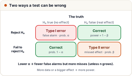
- Type I error (false positive) — you "find" an effect that isn't there. Its probability is α (5% if α = 0.05).
- Type II error (false negative) — you miss a real effect. Its probability is β.
- Power = 1 − β — the chance of detecting a real effect. It grows with sample size and with the size of the effect.
Lowering α to 0.01 cuts false alarms but increases misses, unless you collect more data.
6. The multiple-testing trap
Test 20 things that have no real effect at α = 0.05 and you still expect about one "significant" result:
alpha, tests = 0.05, 20
print(f"chance of at least one false positive: {1 - (1 - alpha) ** tests:.0%}")
print(f"Bonferroni-corrected alpha per test: {alpha / tests}")
chance of at least one false positive: 64%
Bonferroni-corrected alpha per test: 0.0025
If you check many metrics, segments or features, either correct for it (the simple Bonferroni correction divides α by the number of tests) or decide the one main metric before the experiment.
Finally, significant is not the same as important. With a million users, a 0.01-mark difference can have p < 0.001 and still not matter to anyone. Always report the size of the effect (with a confidence interval) next to the p-value.
Common mistakes
- Saying "p > 0.05, so there is no difference" — you only failed to find one.
- Using an independent-groups test on before/after data from the same people.
- Claiming causation from groups that chose themselves.
- Testing many things and reporting only the one with p < 0.05.
- Reporting p-values without the effect size.
Quick recap
- Steps: H₀, H₁, α (before looking), statistic and p-value, decision.
- Two groups → Welch's t-test; same people twice → paired test; counts in a table → chi-square.
- A permutation test builds the "no effect" distribution by shuffling labels or signs.
- Type I = false alarm (α); Type II = missed effect (β); power = 1 − β.
- Correct for multiple tests, and report effect size, not just p.