AdvancedPython for Data Science & Machine Learning · Lesson 14 of 15 · Updated ·
Sampling, Standard Error and Confidence Intervals — How Sure Is Your Average?
You almost never measure everyone. A college surveys 100 students, not all 5,000; an app tests a feature on 2% of users. The number you get is an estimate. A good data scientist always says how uncertain it is: "average study time is 72 minutes, give or take 8" is far more useful than "72".
1. Population, sample and the wobble
- Population — everyone you care about (all 5,000 students).
- Sample — the ones you actually measured (100 students).
- Parameter — the true value in the population (the real average). Usually unknown.
- Statistic — the value computed from the sample (the sample average). It changes from sample to sample.
We can see this with a simulated population whose true answer we know:
import numpy as np

rng = np.random.default_rng(42)
population = rng.gamma(shape=2, scale=36, size=50_000)      # daily study minutes: skewed, most study little
print("true population mean:", population.mean().round(1))

for i in range(4):
    sample = rng.choice(population, size=100, replace=False)
    print(f"sample {i + 1}: mean of 100 students = {sample.mean():.1f}")
true population mean: 71.9
sample 1: mean of 100 students = 87.4
sample 2: mean of 100 students = 76.2
sample 3: mean of 100 students = 82.0
sample 4: mean of 100 students = 76.0
Four honest surveys, four different answers. None of them is "wrong" — that variation is called sampling error, and it is unavoidable. What we can do is measure it.
2. Standard error: how much a sample mean wobbles
If we repeated the survey many times, the sample means would form their own distribution — the sampling distribution. Its standard deviation is the standard error (SE):
SE = s ÷ √n, where s is the standard deviation of the data and n is the sample size.
import numpy as np

rng = np.random.default_rng(42)
population = rng.gamma(shape=2, scale=36, size=50_000)

for n in (25, 100, 400):
    means = [rng.choice(population, size=n).mean() for _ in range(3000)]
    print(f"n = {n:3d}: spread of 3000 sample means = {np.std(means):.2f}   formula sd/sqrt(n) = {population.std() / np.sqrt(n):.2f}")
n =  25: spread of 3000 sample means = 10.02   formula sd/sqrt(n) = 10.21
n = 100: spread of 3000 sample means = 5.09   formula sd/sqrt(n) = 5.11
n = 400: spread of 3000 sample means = 2.56   formula sd/sqrt(n) = 2.55
The formula matches the simulation. Notice the √n: four times more students only halves the error. Going from 100 to 400 students costs four times as much and buys half the uncertainty — a real trade-off when planning a survey.
3. The central limit theorem
The study-time data is skewed (a long tail of students who study a lot). Yet the sample means form a symmetric, bell-shaped curve around the true mean:
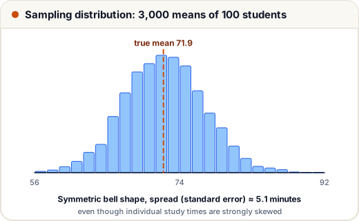
This is the central limit theorem (CLT): for a large enough sample (a common rule of thumb is 30 or more, more for very skewed data), the mean of the sample is approximately normally distributed, whatever the shape of the original data. It is the reason the normal distribution appears in so many formulas, including the next one.
4. A 95% confidence interval
Because sample means are roughly normal, about 95% of them land within 1.96 standard errors of the true mean. Turned around, from one sample we can write:
95% CI = sample mean ± 1.96 × SE
import numpy as np

rng = np.random.default_rng(42)
population = rng.gamma(shape=2, scale=36, size=50_000)
true_mean = population.mean()

sample = rng.choice(population, size=100, replace=False)
se = sample.std(ddof=1) / np.sqrt(len(sample))       # ddof=1: the sample standard deviation
low, high = sample.mean() - 1.96 * se, sample.mean() + 1.96 * se
print(f"estimate {sample.mean():.1f} minutes, 95% CI {low:.1f} to {high:.1f}")

hits = 0
for _ in range(1000):                                 # repeat the whole survey 1000 times
    s = rng.choice(population, size=100, replace=False)
    m, e = s.mean(), 1.96 * s.std(ddof=1) / np.sqrt(100)
    hits += (m - e) <= true_mean <= (m + e)
print(f"intervals that contained the true mean: {hits / 10:.1f}%")
estimate 87.4 minutes, 95% CI 73.6 to 101.2
intervals that contained the true mean: 93.6%
Look at both lines. This particular sample (the same first sample as in section 1) was an unlucky one: its interval, 73.6 to 101.2, misses the true mean of 71.9. That happens to about 1 sample in 20 — and you never know which one you have. Over 1,000 repeated surveys, 93.6% of the intervals contained the true mean: close to the promised 95%, a little lower because the data is strongly skewed and 100 is only a moderate sample size.
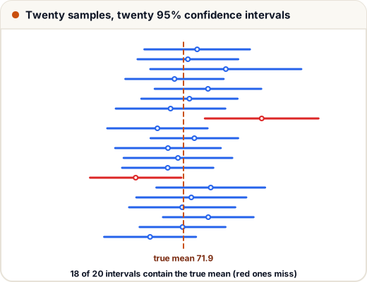
What "95% confidence" really means: the method catches the true value in about 95% of repeated surveys. It does not mean "there is a 95% chance the true mean is in this particular interval" — the true mean is fixed; it is either inside or not. In practice, read it as "our estimate is probably off by no more than this much".
5. The bootstrap: a confidence interval for anything
The ± 1.96 × SE formula is for means. What about the median delivery time, or a 90th percentile? The bootstrap needs no formula: resample your own sample with replacement many times, compute the statistic each time, and take the middle 95% of the results.
import numpy as np

rng = np.random.default_rng(7)
delivery_minutes = rng.gamma(shape=3, scale=10, size=60).round()     # one week's sample of 60 orders

medians = [np.median(rng.choice(delivery_minutes, size=60, replace=True)) for _ in range(5000)]
low, high = np.percentile(medians, [2.5, 97.5])
print("sample median:", np.median(delivery_minutes))
print(f"95% bootstrap CI for the median: {low} to {high}")
sample median: 25.0
95% bootstrap CI for the median: 20.0 to 28.0
The bootstrap treats your sample as a small copy of the population. It works for medians, percentiles, ratios and model scores — that's why it is used so widely in data science.
6. How many people should a survey ask?
For a proportion (for example "what share of students want weekend classes?"), the margin of error at 95% confidence is about 1.96 × √(p(1 − p) ÷ n). Taking the worst case p = 0.5 and solving for n:
import math

def sample_size(margin, p=0.5, z=1.96):
    return math.ceil(z ** 2 * p * (1 - p) / margin ** 2)

for margin in (0.10, 0.05, 0.03, 0.01):
    print(f"margin ±{margin:.0%}: ask about {sample_size(margin):,} people")
margin ±10%: ask about 97 people
margin ±5%: ask about 385 people
margin ±3%: ask about 1,068 people
margin ±1%: ask about 9,604 people
Halving the margin needs four times the people — the √n rule again. (This simple formula assumes a population much larger than the sample, chosen at random.)
7. Sampling bias: a big sample can still be wrong
All the maths above assumes a random sample. No formula fixes a biased one:
| Bias | Example |
|---|---|
| Selection bias | surveying only students in the library about study hours |
| Non-response bias | only happy customers fill in the feedback form |
| Survivorship bias | studying only placed alumni to learn "what works" |
| Convenience sampling | asking your own WhatsApp group and calling it "students" |
A random sample of 400 beats a biased sample of 40,000.
Common mistakes
- Reporting an estimate without any measure of uncertainty.
- Thinking a 95% CI means a 95% chance for this specific interval.
- Expecting double the data to halve the error (it takes four times).
- Using the normal-formula interval for a median or percentile — use the bootstrap.
- Trusting a huge but biased sample.
Quick recap
- A sample statistic estimates a population parameter and varies from sample to sample.
- Standard error = s ÷ √n; quadruple n to halve it.
- Central limit theorem: sample means are roughly normal for large enough samples.
- 95% CI ≈ mean ± 1.96 × SE; the bootstrap gives intervals for any statistic.
- Margin ±5% on a proportion needs about 385 random people; no sample size cures bias.