AdvancedPython for Data Science & Machine Learning · Lesson 21 of 21 · Updated ·
Neural Networks from Scratch — Neurons, Layers, Activations and Backpropagation in NumPy
Image recognition, speech-to-text and large language models are all neural networks. They look complex, but they are built from the two things you already wrote in the last lessons: a weighted sum followed by a squashing function (logistic regression), and gradient descent. This lesson builds a tiny network that solves a problem logistic regression cannot, and trains it with backpropagation.
1. A problem a straight line cannot solve
Many Indian homes have a staircase light with one switch at the bottom and one at the top. Flipping either switch changes the light. So the light is ON when exactly one switch is up:
| bottom switch | top switch | light |
|---|---|---|
| 0 | 0 | off (0) |
| 0 | 1 | on (1) |
| 1 | 0 | on (1) |
| 1 | 1 | off (0) |
This rule is called XOR (exclusive OR). Logistic regression draws a single straight line to separate 1s from 0s. Try it:
import numpy as np

X = np.array([[0, 0], [0, 1], [1, 0], [1, 1]], dtype=float)
y = np.array([0, 1, 1, 0], dtype=float)

w, b = np.zeros(2), 0.0
for _ in range(5000):
    p = 1 / (1 + np.exp(-(X @ w + b)))
    w -= 0.5 * X.T @ (p - y) / 4
    b -= 0.5 * np.mean(p - y)

print("probabilities:", p.round(2))
print("accuracy:", np.mean((p >= 0.5) == y))
probabilities: [0.5 0.5 0.5 0.5]
accuracy: 0.5
It gives up and says 0.5 for every case. No straight line can put (0,1) and (1,0) on one side and (0,0) and (1,1) on the other: draw the four corners of a square and try it. We need a model that can make a bent boundary.
2. Neurons and layers
A neuron does what logistic regression does: multiply the inputs by weights, add a bias, and pass the result through an activation function. A layer is several neurons that all look at the same inputs. A neural network feeds the outputs of one layer into the next.
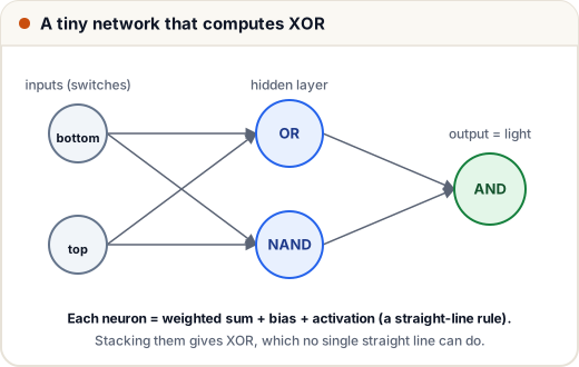
XOR can be built from simpler pieces: it is "at least one switch is up" (OR) and "not both are up" (NAND). Each of those is a straight-line rule, so one neuron can learn each. A second-layer neuron combines them with AND. Here are hand-chosen weights that do exactly that:
import numpy as np

def step(z):
    return (z > 0).astype(int)

X = np.array([[0, 0], [0, 1], [1, 0], [1, 1]])

W1 = np.array([[1, -1],          # column 0 = OR neuron, column 1 = NAND neuron
               [1, -1]])
b1 = np.array([-0.5, 1.5])
hidden = step(X @ W1 + b1)

W2 = np.array([1, 1])            # AND of the two hidden neurons
b2 = -1.5
light = step(hidden @ W2 + b2)

for inputs, h, out in zip(X, hidden, light):
    print(inputs, "-> hidden (OR, NAND) =", h, "-> light", out)
[0 0] -> hidden (OR, NAND) = [0 1] -> light 0
[0 1] -> hidden (OR, NAND) = [1 1] -> light 1
[1 0] -> hidden (OR, NAND) = [1 1] -> light 1
[1 1] -> hidden (OR, NAND) = [1 0] -> light 0
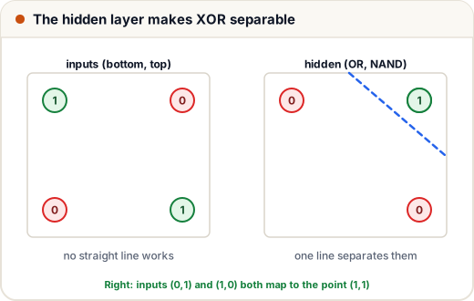
The hidden layer turns the inputs into new features (OR and NAND) in which the problem is separable by a straight line. That is the core idea of deep learning: each layer learns useful features for the next one. In real networks nobody chooses the weights by hand; they are learned.
3. Why the activation function matters
Without an activation function, a layer is just a matrix multiplication, and two matrix multiplications in a row equal one matrix multiplication. So a 10-layer network with no activations is no more powerful than logistic regression.
import numpy as np

rng = np.random.default_rng(0)
x = rng.normal(size=(3, 2))
W1, W2 = rng.normal(size=(2, 4)), rng.normal(size=(4, 1))

two_layers = (x @ W1) @ W2           # two linear layers, no activation
one_layer = x @ (W1 @ W2)            # a single combined layer
print("same result:", np.allclose(two_layers, one_layer))
same result: True
The non-linear activation between layers is what lets the network bend its boundary. Common choices:
| Activation | Formula | Output range | Typical use |
|---|---|---|---|
| Sigmoid | 1 / (1 + e^(−z)) | 0 to 1 | output layer for yes/no |
| tanh | (e^z − e^(−z)) / (e^z + e^(−z)) | −1 to 1 | small networks, older RNNs |
| ReLU | max(0, z) | 0 to ∞ | hidden layers of most modern networks |
| Softmax | e^(zᵢ) / Σ e^(zⱼ) | probabilities that sum to 1 | output layer for many classes |
ReLU is the default for hidden layers in large networks because it is cheap and its gradient does not shrink towards zero for positive inputs, which helps deep networks train.
4. Training: forward pass, backward pass, update
Training repeats three steps:
- Forward pass: compute the prediction layer by layer.
- Backward pass (backpropagation): use the chain rule of calculus to find how much each weight contributed to the loss, starting from the output and moving backwards.
- Update: gradient descent on every weight.
For our network (2 inputs → 3 tanh neurons → 1 sigmoid output, trained with log loss), the backward pass is four lines. The output error p − y is the same expression you saw in logistic regression; it is passed back through W2, multiplied by the slope of tanh, which is 1 − h².
import numpy as np

X = np.array([[0, 0], [0, 1], [1, 0], [1, 1]], dtype=float)
y = np.array([[0], [1], [1], [0]], dtype=float)

def sigmoid(z):
    return 1 / (1 + np.exp(-z))

rng = np.random.default_rng(0)
W1, b1 = rng.normal(0, 1, (2, 3)), np.zeros(3)      # input -> hidden (3 neurons)
W2, b2 = rng.normal(0, 1, (3, 1)), np.zeros(1)      # hidden -> output
lr = 1.0

for epoch in range(3001):
    # forward pass
    h = np.tanh(X @ W1 + b1)
    p = sigmoid(h @ W2 + b2)
    loss = -np.mean(y * np.log(p) + (1 - y) * np.log(1 - p))
    # backward pass (chain rule)
    d_out = (p - y) / len(X)
    dW2, db2 = h.T @ d_out, d_out.sum(axis=0)
    d_hidden = d_out @ W2.T * (1 - h ** 2)
    dW1, db1 = X.T @ d_hidden, d_hidden.sum(axis=0)
    # update
    W1 -= lr * dW1; b1 -= lr * db1
    W2 -= lr * dW2; b2 -= lr * db2
    if epoch in (0, 300, 3000):
        print(f"epoch {epoch:4d}: loss = {loss:.4f}")

print("predictions:", p.ravel().round(3))
epoch    0: loss = 0.7435
epoch  300: loss = 0.0103
epoch 3000: loss = 0.0008
predictions: [0.    0.999 0.999 0.001]
The loss falls from about 0.7 (guessing) to almost 0, and the predictions match the staircase light: off, on, on, off. The network found its own version of the OR/NAND trick.
5. Random starts and local minima
Neural networks start from random weights. Run the same code with different seeds and most runs succeed, but not all:
import numpy as np

X = np.array([[0, 0], [0, 1], [1, 0], [1, 1]], dtype=float)
y = np.array([[0], [1], [1], [0]], dtype=float)

def train(seed):
    rng = np.random.default_rng(seed)
    W1, b1 = rng.normal(0, 1, (2, 3)), np.zeros(3)
    W2, b2 = rng.normal(0, 1, (3, 1)), np.zeros(1)
    for _ in range(3001):
        h = np.tanh(X @ W1 + b1)
        p = 1 / (1 + np.exp(-(h @ W2 + b2)))
        d_out = (p - y) / 4
        d_hidden = d_out @ W2.T * (1 - h ** 2)
        W2 -= h.T @ d_out; b2 -= d_out.sum(axis=0)
        W1 -= X.T @ d_hidden; b1 -= d_hidden.sum(axis=0)
    return p.ravel().round(2)

for seed in range(4):
    print("seed", seed, "->", train(seed))
seed 0 -> [0. 1. 1. 0.]
seed 1 -> [0. 1. 1. 0.]
seed 2 -> [0.  0.5 1.  0.5]
seed 3 -> [0. 1. 1. 0.]
Seed 2 got stuck: it solved two of the four cases and is unsure (0.5) about the others. The loss surface of a neural network is not one smooth bowl; it has flat regions and local minima. Practical fixes include using more hidden neurons than the bare minimum, better starting weights, and improved optimisers such as Adam. Large networks are much less likely to get stuck badly, which is one reason they are made big.
6. From scratch to real frameworks
Real projects use PyTorch, TensorFlow/Keras or JAX. They give you:
- Automatic differentiation: you write only the forward pass; the framework computes the backward pass for you.
- GPUs: fast matrix multiplication on millions of weights.
- Ready layers and optimisers:
Linear,Conv2d,ReLU,Adam, mini-batch data loaders.
The concepts do not change: layers, activations, a loss, backpropagation and gradient descent. Knowing what happens inside makes debugging far easier when a loss refuses to fall.
Common mistakes
- Leaving out the activation function, so the whole network collapses into one linear layer.
- Starting all weights at zero. Every hidden neuron then computes the same thing and receives the same update, so they never become different. Start with small random values.
- Using a learning rate that is too large, so the loss jumps around or becomes
nan. - Using sigmoid in every hidden layer of a deep network; its gradient becomes tiny and early layers learn very slowly (the vanishing gradient problem). Prefer ReLU.
- Judging a network from one run. Try more than one random seed.
Quick recap
- A neuron = weighted sum + bias + activation; layers of neurons form a network.
- One straight boundary cannot solve XOR; a hidden layer creates new features that can.
- Activation functions provide the non-linearity; without them, many layers equal one.
- Training = forward pass, backpropagation (chain rule), gradient descent update.
- Random starts can land in poor local minima; frameworks automate the backward pass.