AdvancedPython for Data Science & Machine Learning · Lesson 16 of 21 · Updated ·
Feature Engineering — Encoding Categories, Scaling, Log Transforms, Binning and Date Features
Models only see numbers. Feature engineering is the work of turning raw columns — text categories, dates, rupee amounts, counts — into numbers that carry the right meaning. On tabular data, good features usually improve a model more than switching to a fancier algorithm.
1. Categories: one-hot or ordinal?
A model can't multiply "CSE" by a coefficient. There are two main ways to turn categories into numbers, and choosing the wrong one quietly misleads the model.
- Ordinal encoding — map categories to 1, 2, 3… only when they have a real order (year of study, small < medium < large, grade C < B < A).
- One-hot encoding — one 0/1 column per category, for categories with no order (branch, city, payment method).
import pandas as pd

df = pd.DataFrame({
    "name": ["Asha", "Ravi", "Neha", "Arjun"],
    "branch": ["CSE", "ECE", "CSE", "ME"],
    "year": ["2nd", "4th", "3rd", "1st"],
})
year_order = {"1st": 1, "2nd": 2, "3rd": 3, "4th": 4}       # a real order: ordinal is fine
df["year_num"] = df["year"].map(year_order)

encoded = pd.get_dummies(df, columns=["branch"], dtype=int)  # no order: one-hot
print(encoded.drop(columns="year").to_string(index=False))
 name  year_num  branch_CSE  branch_ECE  branch_ME
 Asha         2           1           0          0
 Ravi         4           0           1          0
 Neha         3           1           0          0
Arjun         1           0           0          1
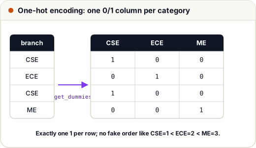
Why not just map CSE = 1, ECE = 2, ME = 3? Because a linear model would then believe ME is "three times" CSE and that ECE lies "between" them. One-hot columns make no such claim.
Two practical warnings:
- Many categories (5,000 colleges, 20,000 pin codes) explode into thousands of columns. Group rare ones into "Other", or use frequency/target encoding with care.
- New categories at prediction time (a branch never seen in training) must be handled — scikit-learn's
OneHotEncoder(handle_unknown="ignore")does this, as shown in the pipelines lesson.
2. Scaling, written by hand
Features often live on very different scales: CGPA from 0 to 10, an aptitude score from 0 to 100, coding minutes per week from 0 to 1,000. Two common fixes:
| Method | Formula | Result |
|---|---|---|
| Min-max scaling | (x − min) ÷ (max − min) | values between 0 and 1 |
| Standardisation (z-score) | (x − mean) ÷ std | mean 0, standard deviation 1 |
The golden rule: learn the min, max, mean and std from the training data only, then apply those same numbers to test data and to new data.
import numpy as np

train_minutes = np.array([120, 300, 450, 800, 200, 650])     # coding minutes per week (training rows)
new_minutes = np.array([500, 1200])                           # two new students

lo, hi = train_minutes.min(), train_minutes.max()
mean, std = train_minutes.mean(), train_minutes.std()
print("min-max  train:", ((train_minutes - lo) / (hi - lo)).round(2))
print("min-max  new:  ", ((new_minutes - lo) / (hi - lo)).round(2))
print("z-score  new:  ", ((new_minutes - mean) / std).round(2))
min-max  train: [0.   0.26 0.49 1.   0.12 0.78]
min-max  new:   [0.56 1.59]
z-score  new:   [0.33 3.22]
Notice the new student with 1,200 minutes gets a min-max value above 1. That's correct behaviour — the training range is not a law. What would be wrong is recomputing min and max using the test data: that leaks test information into training (the leakage section of the pipelines lesson).
3. Why scaling changes the answer: nearest neighbours
k-nearest neighbours (k-NN) classifies a new point by looking at the k most similar training points, using distance. If one feature has much bigger numbers, it decides the distance almost alone.
import numpy as np

# cgpa, aptitude score (0-100), coding minutes per week
students = np.array([[9.1, 62, 300],
                     [6.2, 88, 320],
                     [8.8, 85, 420]])
names = ["Asha", "Ravi", "Sara"]
new = np.array([8.9, 86, 330])

def nearest(data, point):
    dist = np.sqrt(((data - point) ** 2).sum(axis=1))
    return names[dist.argmin()], dist.round(2)

print("raw:   ", nearest(students, new))
mean, std = students.mean(axis=0), students.std(axis=0)
print("scaled:", nearest((students - mean) / std, (new - mean) / std))
raw:    ('Ravi', array([38.42, 10.55, 90.01]))
scaled: ('Sara', array([2.15, 2.09, 1.72]))
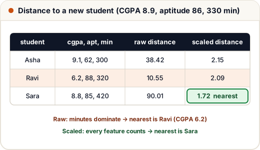
On raw numbers, Sara's 90-minute difference in coding time outweighs everything else, even though her CGPA (8.8) and aptitude (85) almost equal the new student's — so the new student (CGPA 8.9) is matched with Ravi (CGPA 6.2). After scaling, each feature counts on a comparable scale and Sara becomes the nearest neighbour. Distance-based and gradient-based models (k-NN, k-means, SVM, logistic regression with regularisation, neural networks) need scaling; decision trees do not, because they only compare values within one feature at a time.
4. Skewed numbers: the log transform
Money, follower counts and time-on-app are usually right-skewed: most values are small and a few are huge. A log transform pulls the long tail in, so a few extreme rows don't dominate:
import numpy as np

monthly_spend = np.array([120, 250, 300, 180, 90, 400, 220, 15000, 260, 30000])   # rupees
logged = np.log1p(monthly_spend)          # log(1 + x): safe when x is 0
print("raw:    mean", monthly_spend.mean(), " median", np.median(monthly_spend))
print("logged: mean", logged.mean().round(2), " median", np.median(logged).round(2))
print("back to rupees:", np.expm1(np.median(logged)).round())
raw:    mean 4682.0  median 255.0
logged: mean 6.26  median 5.54
back to rupees: 255.0
Before the transform the mean (₹4,682) is about 18 times the median (₹255) because of two big spenders; after it, the mean and median are much closer. Use np.log1p (not np.log) so zero values don't become minus infinity, and np.expm1 to convert predictions back.
5. Binning, ratios and dates
Some of the most useful features are made by combining or reshaping columns with domain knowledge:
import pandas as pd

orders = pd.DataFrame({
    "placed_at": pd.to_datetime(["2026-03-06 21:40", "2026-03-07 13:05", "2026-03-09 08:15", "2026-03-08 22:30"]),
    "problems_solved": [45, 3, 120, 60],
    "problems_tried": [50, 20, 150, 61],
    "age": [19, 23, 31, 20],
})
orders["weekday"] = orders["placed_at"].dt.day_name()
orders["is_weekend"] = orders["placed_at"].dt.dayofweek >= 5
orders["hour"] = orders["placed_at"].dt.hour
orders["solve_rate"] = (orders["problems_solved"] / orders["problems_tried"]).round(2)
orders["age_group"] = pd.cut(orders["age"], bins=[0, 21, 25, 100], labels=["≤21", "22-25", "26+"])
print(orders.drop(columns=["placed_at", "problems_solved", "problems_tried"]).to_string(index=False))
 age  weekday  is_weekend  hour  solve_rate age_group
  19   Friday       False    21        0.90       ≤21
  23 Saturday        True    13        0.15     22-25
  31   Monday       False     8        0.80       26+
  20   Sunday        True    22        0.98       ≤21
| Feature type | Example | Why it helps |
|---|---|---|
| Date parts | weekday, hour, month, is_weekend | behaviour follows the calendar |
| Ratios | solved ÷ tried, fee paid ÷ fee due | compares fairly across very active and less active users |
| Binning | age groups, CGPA bands | captures steps, and is easy to explain |
| Counts / recency | orders in last 30 days, days since last login | recent behaviour predicts the next action |
A raw timestamp like 2026-03-06 21:40 is nearly useless to a model; "Friday, 21:00, weekday" is meaningful.
6. Where feature engineering goes wrong
- Leakage features — anything known only after the outcome (e.g. "offer_letter_date" when predicting placement). Ask: would I have this value at prediction time?
- Fitting on all data — scaling or encoding statistics must come from the training split only.
- Hand-made features in a notebook only — the same code must run in production. Put it in a function or a scikit-learn
Pipelineso training and prediction use identical steps.
Common mistakes
- Ordinal-encoding categories that have no order (branch → 1, 2, 3).
- Scaling with statistics computed on the whole dataset, including test rows.
- Forgetting to scale before k-NN or k-means.
- Using
np.logon data containing zeros instead ofnp.log1p. - Feeding raw timestamps or IDs to a model as if they were numbers.
Quick recap
- One-hot for unordered categories; ordinal mapping only for real orders.
- Min-max → 0 to 1; z-score → mean 0, std 1; always fit on training data only.
- Distance-based models need scaling; trees don't.
- Log-transform right-skewed values; build date parts, ratios and bins from domain knowledge.
- Every feature must be available at prediction time and computed the same way in production.