AdvancedPython for Data Science & Machine Learning · Lesson 19 of 21 · Updated ·
Logistic Regression from Scratch — Sigmoid, Log Loss, Gradient Descent and the Decision Threshold
In the classification lesson, scikit-learn's LogisticRegression predicted whether a student gets placed. In the last lesson you wrote gradient descent for a straight line. Put the two together and you can build logistic regression yourself in about 20 lines. Doing it once makes three interview favourites easy to explain: the sigmoid, log loss, and the decision threshold.
1. The problem: predicting yes or no
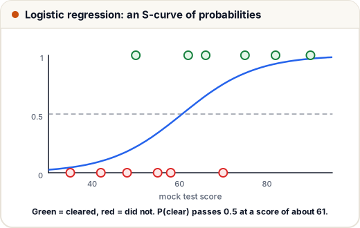
Data: the score of 12 students in a mock placement test (out of 100) and whether they cleared the real company test (1 = cleared, 0 = not). This is practice data.
We want a probability: "a student with 62 marks has a 70% chance of clearing". A straight line w × score + b cannot give that. It goes below 0 and above 1, and a probability of 1.3 or −0.2 makes no sense.
import numpy as np

score = np.array([35, 42, 48, 50, 55, 58, 62, 66, 70, 75, 82, 90], dtype=float)
cleared = np.array([0, 0, 0, 1, 0, 0, 1, 1, 0, 1, 1, 1], dtype=float)

w, b = np.polyfit(score, cleared, 1)          # an ordinary straight line
for s in (20, 60, 110):
    print(f"score {s:3d}: line says {w * s + b:+.2f}")
score  20: line says -0.31
score  60: line says +0.48
score 110: line says +1.47
The line gives values outside 0 to 1. We need a function that squeezes any number into that range.
2. The sigmoid function
The sigmoid (also called the logistic function) is σ(z) = 1 / (1 + e^(−z)).
- Large positive
z→ close to 1. - Large negative
z→ close to 0. z = 0→ exactly 0.5.
import numpy as np

def sigmoid(z):
    return 1 / (1 + np.exp(-z))

for z in (-6, -2, 0, 2, 6):
    print(f"z = {z:+d}  ->  sigmoid = {sigmoid(z):.3f}")
z = -6  ->  sigmoid = 0.002
z = -2  ->  sigmoid = 0.119
z = +0  ->  sigmoid = 0.500
z = +2  ->  sigmoid = 0.881
z = +6  ->  sigmoid = 0.998
Logistic regression is just: probability = sigmoid(w × x + b). The straight line is still inside; the sigmoid bends it into an S-shape between 0 and 1. The value z = w × x + b is called the log-odds (or logit).
3. Log loss: the right way to measure a wrong probability
For regression we used mean squared error. For probabilities we use log loss (also called binary cross-entropy):
- If the true answer is 1, the loss is
−log(p). - If the true answer is 0, the loss is
−log(1 − p).
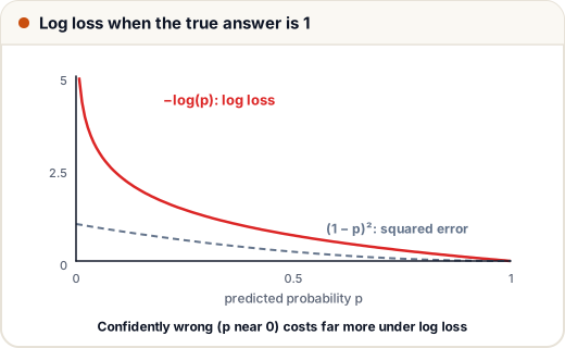
So the loss is small when you give the true answer a high probability, and it grows without limit when you are confidently wrong.
import numpy as np

def log_loss_one(y, p):
    return -(y * np.log(p) + (1 - y) * np.log(1 - p))

print("Student actually cleared (y = 1):")
for p in (0.99, 0.7, 0.5, 0.1, 0.01):
    print(f"  model said p = {p:4}: log loss = {log_loss_one(1, p):.3f}   squared error = {(1 - p) ** 2:.3f}")
Student actually cleared (y = 1):
  model said p = 0.99: log loss = 0.010   squared error = 0.000
  model said p =  0.7: log loss = 0.357   squared error = 0.090
  model said p =  0.5: log loss = 0.693   squared error = 0.250
  model said p =  0.1: log loss = 2.303   squared error = 0.810
  model said p = 0.01: log loss = 4.605   squared error = 0.980
Compare the last row. A model that said "1% chance" for a student who cleared is badly wrong. Squared error caps that mistake at about 1, but log loss gives 4.6, a much stronger push to fix it. Log loss also gives a smooth bowl-shaped surface for gradient descent, so training is reliable.
4. Training with gradient descent
The gradient of log loss has a neat form, the same shape as for linear regression:
- ∂loss/∂w = mean((p − y) × x)
- ∂loss/∂b = mean(p − y)
We standardise the score first (subtract the mean, divide by the standard deviation), because the last lesson showed that scaled features train much faster.
import numpy as np

score = np.array([35, 42, 48, 50, 55, 58, 62, 66, 70, 75, 82, 90], dtype=float)
cleared = np.array([0, 0, 0, 1, 0, 0, 1, 1, 0, 1, 1, 1], dtype=float)

def sigmoid(z):
    return 1 / (1 + np.exp(-z))

mean, std = score.mean(), score.std()
x = (score - mean) / std

w, b, lr = 0.0, 0.0, 0.5
for epoch in range(1001):
    p = sigmoid(w * x + b)
    loss = -np.mean(cleared * np.log(p) + (1 - cleared) * np.log(1 - p))
    w -= lr * np.mean((p - cleared) * x)
    b -= lr * np.mean(p - cleared)
    if epoch in (0, 50, 1000):
        print(f"epoch {epoch:4d}: log loss = {loss:.4f}")

print(f"w = {w:.3f}, b = {b:.3f}  (on the standardised score)")
for s in (45, 60, 80):
    print(f"mock score {s}: P(clear) = {sigmoid(w * (s - mean) / std + b):.2f}")
epoch    0: log loss = 0.6931
epoch   50: log loss = 0.4622
epoch 1000: log loss = 0.4613
w = 1.873, b = 0.055  (on the standardised score)
mock score 45: P(clear) = 0.13
mock score 60: P(clear) = 0.48
mock score 80: P(clear) = 0.91
At epoch 0 every prediction is 0.5, so the loss is log(2) ≈ 0.693, the loss of pure guessing. Training brings it down, and the model now gives sensible probabilities: low for 45 marks, high for 80.
5. From probability to decision: the threshold
The model outputs a probability. To act, you pick a threshold: predict "will clear" if p ≥ threshold. The default 0.5 is not always right.
import numpy as np

score = np.array([35, 42, 48, 50, 55, 58, 62, 66, 70, 75, 82, 90], dtype=float)
cleared = np.array([0, 0, 0, 1, 0, 0, 1, 1, 0, 1, 1, 1])

def sigmoid(z):
    return 1 / (1 + np.exp(-z))

mean, std = score.mean(), score.std()
x = (score - mean) / std
w = b = 0.0
for _ in range(1001):
    p = sigmoid(w * x + b)
    w -= 0.5 * np.mean((p - cleared) * x)
    b -= 0.5 * np.mean(p - cleared)
p = sigmoid(w * x + b)

print("threshold  predicted-yes  precision  recall")
for t in (0.3, 0.5, 0.7):
    pred = (p >= t).astype(int)
    tp = int(((pred == 1) & (cleared == 1)).sum())
    precision = tp / pred.sum()
    recall = tp / cleared.sum()
    print(f"   {t}          {pred.sum():2d}          {precision:.2f}      {recall:.2f}")
threshold  predicted-yes  precision  recall
   0.3           8          0.62      0.83
   0.5           6          0.83      0.83
   0.7           4          0.75      0.50
- Lower threshold → more students flagged "will clear" → higher recall (you miss fewer real successes) but lower precision (more false alarms).
- Higher threshold → fewer, surer predictions → usually higher precision, lower recall.
With only 12 students the numbers jump around: at 0.7 precision actually dips to 0.75, because one of the four flagged students (70 marks) did not clear. On real data with thousands of rows the trade-off is much smoother.
Choose the threshold by the cost of each mistake. Suppose a college uses the model to give a few scarce company-referral slots to students likely to clear: a false alarm wastes a slot, so a higher threshold makes sense. If instead it is used to find students likely to clear and invite them to a free advanced workshop, missing a good student is the bigger loss, so a lower threshold makes sense. The threshold is a business decision, not a property of the model.
6. Reading the weights as odds
Odds = p / (1 − p). A probability of 0.8 is odds of 4 (4 to 1). In logistic regression, increasing a feature by 1 unit multiplies the odds by e^w.
In our model the feature is the standardised score, so one unit is one standard deviation (about 15.7 marks):
import numpy as np

score = np.array([35, 42, 48, 50, 55, 58, 62, 66, 70, 75, 82, 90], dtype=float)
cleared = np.array([0, 0, 0, 1, 0, 0, 1, 1, 0, 1, 1, 1], dtype=float)
mean, std = score.mean(), score.std()
x = (score - mean) / std
w = b = 0.0
for _ in range(1001):
    p = 1 / (1 + np.exp(-(w * x + b)))
    w -= 0.5 * np.mean((p - cleared) * x)
    b -= 0.5 * np.mean(p - cleared)

print(f"one standard deviation = {std:.1f} marks")
print(f"odds multiply by e^w = {np.exp(w):.2f} for each extra {std:.1f} marks")
one standard deviation = 15.7 marks
odds multiply by e^w = 6.51 for each extra 15.7 marks
This is why logistic regression is popular in banking and healthcare: each weight has a clear meaning that you can explain to a manager.
Common mistakes
- Using a straight line (linear regression) for yes/no targets and treating its output as a probability.
- Using mean squared error instead of log loss to train a classifier.
- Always using 0.5 as the threshold without thinking about the cost of each kind of mistake.
- Forgetting to scale features before gradient descent.
- Reading a weight as "adds w to the probability". It multiplies the odds by e^w; the change in probability depends on where you start.
- Taking
log(0)when a probability becomes exactly 0 or 1. Libraries clip p to a tiny range such as [1e-15, 1 − 1e-15] to avoid this.
Quick recap
- Logistic regression: p = sigmoid(w·x + b); the sigmoid maps any number into (0, 1).
- Train it by minimising log loss with gradient descent; the gradient is mean((p − y) × x).
- Log loss punishes confident wrong answers very strongly.
- The threshold turns probabilities into decisions and trades precision against recall.
- e^w is the odds ratio for a one-unit increase in a feature.