AdvancedPython for Data Science & Machine Learning · Lesson 18 of 21 · Updated ·
Gradient Descent from Scratch — Linear Regression, Loss, Learning Rate and Feature Scaling
In the regression lesson, model.fit() found the best line in one call. What happened inside? For linear regression there is a direct formula, but almost every other model — logistic regression, neural networks, large language models — learns with one idea: gradient descent. Write it once yourself and the rest of machine learning becomes far less mysterious.
1. The loss: a number that says how wrong we are
Data: hours a student studied in the week before a test, and the marks they got (practice data).
A line predicts marks = w × hours + b. The loss measures how bad a choice of w (weight, the slope) and b (bias, the intercept) is. For regression the usual loss is the mean squared error (MSE): the average of (prediction − actual)².
import numpy as np

hours = np.array([1, 2, 3, 4, 5, 6, 7, 8], dtype=float)
marks = np.array([38, 45, 51, 55, 63, 66, 74, 80], dtype=float)

def mse(w, b):
    return np.mean((w * hours + b - marks) ** 2)

for w, b in [(0, 50), (5, 30), (6, 32), (8, 20)]:
    print(f"w={w}, b={b}: MSE = {mse(w, b):.1f}")
w=0, b=50: MSE = 262.0
w=5, b=30: MSE = 47.0
w=6, b=32: MSE = 1.0
w=8, b=20: MSE = 34.0
Learning = finding the w and b with the lowest loss. We could try every combination, but with millions of parameters that's impossible. We need a smarter way to walk downhill.
2. The gradient points uphill — so step the other way
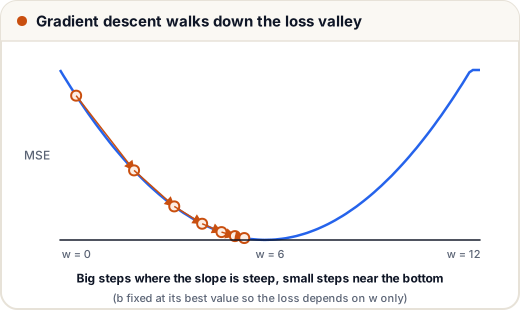
Picture the loss as a valley. The gradient is the slope of the loss with respect to each parameter: it says which direction is uphill and how steep it is. For MSE:
- ∂loss/∂w = 2 × mean((prediction − actual) × hours)
- ∂loss/∂b = 2 × mean(prediction − actual)
Gradient descent repeats one step: parameter = parameter − learning_rate × gradient.
import numpy as np

hours = np.array([1, 2, 3, 4, 5, 6, 7, 8], dtype=float)
marks = np.array([38, 45, 51, 55, 63, 66, 74, 80], dtype=float)

w, b, lr = 0.0, 0.0, 0.02
for epoch in range(2001):
    pred = w * hours + b
    error = pred - marks
    grad_w = 2 * np.mean(error * hours)
    grad_b = 2 * np.mean(error)
    w -= lr * grad_w                    # step DOWNHILL: minus the gradient
    b -= lr * grad_b
    if epoch in (0, 10, 100, 500, 2000):
        print(f"epoch {epoch:4d}: w={w:6.3f} b={b:7.3f} MSE={np.mean(error ** 2):8.2f}")

print("closed-form answer (np.polyfit):", np.polyfit(hours, marks, 1).round(3))
epoch    0: w=11.850 b=  2.360 MSE= 3662.00
epoch   10: w=10.846 b=  4.596 MSE=  165.50
epoch  100: w= 8.282 b= 19.012 MSE=   39.78
epoch  500: w= 5.955 b= 32.091 MSE=    0.96
epoch 2000: w= 5.857 b= 32.643 MSE=    0.89
closed-form answer (np.polyfit): [ 5.857 32.643]
The loss falls quickly at first, then slowly, and gradient descent arrives at the same line as the exact formula: about 5.86 marks per extra hour, starting from about 32.6. (Each full pass over the data is called an epoch.)
Why do the steps shrink by themselves? Near the bottom of the valley the slope is nearly flat, so the gradient — and therefore each step — becomes small.
3. The learning rate: the most important setting
The learning rate (lr) decides the step size. It is a hyperparameter: you choose it, the algorithm doesn't learn it.
import numpy as np

hours = np.array([1, 2, 3, 4, 5, 6, 7, 8], dtype=float)
marks = np.array([38, 45, 51, 55, 63, 66, 74, 80], dtype=float)

def train(lr, epochs=500):
    w = b = 0.0
    for _ in range(epochs):
        error = w * hours + b - marks
        w -= lr * 2 * np.mean(error * hours)
        b -= lr * 2 * np.mean(error)
    return np.mean((w * hours + b - marks) ** 2)

for lr in (0.001, 0.02, 0.04):
    print(f"lr = {lr:5}: MSE after 500 epochs = {train(lr):.4g}")
lr = 0.001: MSE after 500 epochs = 130.5
lr =  0.02: MSE after 500 epochs = 0.9566
lr =  0.04: MSE after 500 epochs = 3.32e+46
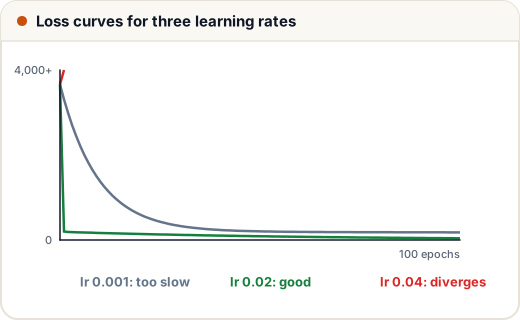
- Too small (0.001): safe but painfully slow — still far from the bottom after 500 epochs.
- Good (0.02): reaches the minimum quickly.
- Too large (0.04): each step jumps past the bottom to a higher point on the other side, and the loss explodes. This is called divergence. If your training loss becomes
infornan, lower the learning rate first.
In practice you try values spaced by about ×3 or ×10 (0.1, 0.03, 0.01, 0.003…) and watch the loss curve.
4. Many features at once (vectorised)
With several features, w becomes a vector and the prediction is a matrix product X @ w + b. The gradient formula stays the same shape:
import numpy as np

rng = np.random.default_rng(1)
n = 200
cgpa = rng.uniform(6, 10, n)
internships = rng.integers(0, 3, n).astype(float)
aptitude = rng.uniform(30, 100, n)
package = 1.0 + 0.8 * cgpa + 0.6 * internships + 0.02 * aptitude + rng.normal(0, 0.3, n)   # LPA, simulated

X = np.column_stack([cgpa, internships, aptitude])
X_scaled = (X - X.mean(axis=0)) / X.std(axis=0)          # standardise each feature

def gradient_descent(X, y, lr, epochs=300):
    w, b = np.zeros(X.shape[1]), 0.0
    for _ in range(epochs):
        error = X @ w + b - y
        w -= lr * 2 * X.T @ error / len(y)
        b -= lr * 2 * error.mean()
    return w, b, np.mean((X @ w + b - y) ** 2)

w, b, loss = gradient_descent(X_scaled, package, lr=0.1)
print("scaled features:   MSE =", round(loss, 4))
w_raw, b_raw, loss_raw = gradient_descent(X, package, lr=0.0001)
print("unscaled features: MSE =", round(loss_raw, 4), "(the largest lr that doesn't diverge here is tiny)")

exact, *_ = np.linalg.lstsq(np.column_stack([X_scaled, np.ones(n)]), package, rcond=None)
print("gradient descent w:", w.round(3), " exact w:", exact[:3].round(3))
scaled features:   MSE = 0.107
unscaled features: MSE = 3.0533 (the largest lr that doesn't diverge here is tiny)
gradient descent w: [0.914 0.511 0.379]  exact w: [0.914 0.511 0.379]
Two lessons in one output:
- With standardised features, gradient descent reaches the exact least-squares answer in 300 epochs.
- With raw features, aptitude (30–100) is much larger than internships (0–2). The valley becomes a long, narrow canyon: a learning rate big enough to make progress along one direction overshoots along another. You are forced to use a tiny learning rate, and after the same 300 epochs the loss is still far from the minimum. Feature scaling makes gradient descent faster and more stable — that's why scaling matters for every gradient-trained model.
5. Batch, stochastic and mini-batch
| Variant | Gradient computed on | Pros | Cons |
|---|---|---|---|
| Batch gradient descent | all rows, every step | smooth, exact direction | slow on big data |
| Stochastic (SGD) | one random row per step | very fast steps, works on streams | noisy path |
| Mini-batch | e.g. 32–512 rows per step | best of both; uses GPUs well | one more setting (batch size) |
Deep learning almost always uses mini-batch gradient descent, usually with improved update rules such as momentum or Adam, which adapt the step size automatically. The core idea is still the update you wrote above.
For plain linear regression, libraries usually use the direct least-squares solution instead (as LinearRegression does); gradient descent shines when no direct formula exists or the data is too big for one.
Common mistakes
- Adding the gradient instead of subtracting it (walking uphill).
- A learning rate so large that the loss explodes to
inf/nan. - Forgetting to scale features before gradient descent.
- Stopping after a fixed number of epochs without looking at the loss curve.
- Updating
wand then using the newwto compute the gradient forbin the same step (compute all gradients first, then update).
Quick recap
- Loss (MSE for regression) measures how wrong the parameters are.
- Gradient = direction of steepest increase; update: parameter −= learning rate × gradient.
- Learning rate: too small is slow, too large diverges; watch the loss curve.
- Vectorised update:
w -= lr * 2 * X.T @ error / n; scale features first. - Batch, stochastic and mini-batch differ only in how many rows each gradient uses.