AdvancedDBMS & SQL · Lesson 23 of 25 · Updated ·
Query Processing and Optimization — Query Trees, Join Algorithms, Cost Estimates and EXPLAIN
SQL is declarative: you say what you want ("names of Pune students"), not how to get it. The database chooses the how — which index to use, which table to read first, which join method. For one query there can be hundreds of possible plans whose run times differ by thousands of times. The part of the DBMS that picks a good one is the query optimizer. Knowing how it thinks helps you write fast queries and answer a common DBMS exam question.
1. The steps of query processing
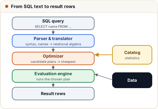
- Parsing and translation — check the syntax, check that the tables and columns exist (using the catalog, the database's data about its own tables), and translate the query into relational algebra.
- Optimization — generate equivalent plans and estimate the cost of each; pick the cheapest.
- Evaluation — the execution engine runs the chosen plan and returns the rows.
An evaluation plan is a relational algebra tree in which every operator is labelled with how it runs: "use index idx_city for this selection", "hash join here".
2. Equivalent expressions and heuristic rules
Many relational algebra expressions give the same answer. For "name and marks of students from Pune":
- Plan A: join
studentswithresults, then keep the Pune rows: σ[city='Pune'](students ⋈ results) - Plan B: keep the Pune students first, then join: σcity='Pune' ⋈ results
Both are correct. Suppose there are 5,000 students spread evenly over 50 cities, each with 2 rows in results:
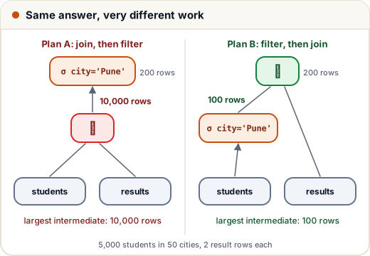
Plan A builds 10,000 intermediate rows and throws 98% of them away. Plan B never creates them. That leads to the classic heuristic rules that optimizers apply first:
| Rule | Why |
|---|---|
| Push selections (σ) down — filter as early as possible | smaller inputs to every later operation |
| Push projections (π) down — drop unneeded columns early | fewer bytes per row to move and sort |
| Combine × with σ into a join | never build a full Cartesian product |
| Do the most selective operations and joins first | keeps intermediate results small |
3. Cost-based optimization
Heuristics alone don't decide between two indexes or two join orders. A cost-based optimizer estimates the cost of each candidate plan, mostly as the number of disk block transfers (and seeks), because reading from disk is far slower than CPU work. To estimate it, the catalog keeps statistics:
| Statistic | Symbol | Example |
|---|---|---|
| number of rows in r | n_r | 5,000 students |
| number of disk blocks of r | b_r | 100 blocks |
| number of distinct values of A in r | V(A, r) | 50 cities |
Selectivity estimate for an equality condition: σA=v returns about n_r / V(A, r) rows, assuming values are evenly spread. Here 5,000 / 50 = 100 Pune students. If real data is skewed (half the students are from one city), the estimate is wrong, which is why databases also keep histograms, and why you run ANALYZE (PostgreSQL, SQLite) or ANALYZE TABLE (MySQL) to refresh statistics after big data changes.
4. Join algorithms and their costs
Joins are usually the most expensive operation, so the method matters. Take r = results (n_r = 10,000 rows in b_r = 400 blocks) and s = students (n_s = 5,000 rows in b_s = 100 blocks), with worst-case memory (one block of each table at a time):
n_r, b_r = 10_000, 400     # results  (outer)
n_s, b_s = 5_000, 100      # students (inner)

costs = {
    'nested loop, results outer':   n_r * b_s + b_r,
    'nested loop, students outer':  n_s * b_r + b_s,
    'block nested loop':            b_r * b_s + b_r,
    'inner table fits in memory':   b_r + b_s,
    'sort-merge (already sorted)':  b_r + b_s,
    'hash join (approx. 3(br+bs))': 3 * (b_r + b_s),
}
for name, c in costs.items():
    print(f'{name:30} {c:>10,} block transfers')
nested loop, results outer      1,000,400 block transfers
nested loop, students outer     2,000,100 block transfers
block nested loop                  40,400 block transfers
inner table fits in memory            500 block transfers
sort-merge (already sorted)           500 block transfers
hash join (approx. 3(br+bs))        1,500 block transfers
| Algorithm | Idea | Best when |
|---|---|---|
| Nested loop | for every row of r, scan all of s | tiny tables; works for any join condition (even <, LIKE) |
| Block nested loop | for every block of r, scan s once | no index, no sort order; far better than plain nested loop |
| Index nested loop | for every row of r, look up matching rows of s through an index on s | an index exists on the inner table's join column |
| Sort-merge join | sort both on the join column, then merge in one pass | inputs already sorted, or output needed sorted; equi-joins only |
| Hash join | build a hash table on the smaller input, probe it with the other | large equi-joins without useful indexes |
For the same join, the worst method needs about 4,000 times as many block transfers as the best one. This is why a missing index or stale statistics can turn a 50 ms query into a minute.
5. Seeing the plan: EXPLAIN
Every major database shows the chosen plan: EXPLAIN in MySQL and PostgreSQL (EXPLAIN ANALYZE also runs the query and shows real times), and EXPLAIN QUERY PLAN in SQLite. The program below asks SQLite for its plans:
import sqlite3

db = sqlite3.connect(':memory:')
db.executescript('''
CREATE TABLE students (roll INTEGER PRIMARY KEY, name TEXT, city TEXT, cgpa REAL);
CREATE TABLE results (roll INTEGER, subject TEXT, marks INTEGER);
''')

def plan(sql):
    for row in db.execute('EXPLAIN QUERY PLAN ' + sql):
        print('  ', row[3])

q = "SELECT name FROM students WHERE city = 'Pune'"
print('No index:')
plan(q)
db.execute('CREATE INDEX idx_city ON students(city)')
print('With index:')
plan(q)
print('Function on the column:')
plan("SELECT name FROM students WHERE lower(city) = 'pune'")
print('Join:')
plan("SELECT s.name, r.marks FROM students s JOIN results r ON r.roll = s.roll")
No index:
   SCAN students
With index:
   SEARCH students USING INDEX idx_city (city=?)
Function on the column:
   SCAN students
Join:
   SCAN r
   SEARCH s USING INTEGER PRIMARY KEY (rowid=?)
How to read it:
SCAN students— a full table scan: every row is read.SEARCH ... USING INDEX idx_city (city=?)— the index is used to jump to matching rows.- With
lower(city), the index is not used: the index storescity, notlower(city). A condition that can use an index is called sargable. Keep indexed columns bare: writecity = 'Pune',order_date >= '2026-01-01', notYEAR(order_date) = 2026. - The join is an index nested loop: scan
results, and for each row look up the student by primary key.
(The exact wording comes from SQLite 3.43 and differs between versions and between database products, but every plan answers the same questions: scan or index, which join method, in what order.)
6. Writing optimizer-friendly SQL
- Select only the columns you need instead of
SELECT *— less data to read and send, and sometimes the index alone can answer (a covering index). - Index the columns used in
WHERE,JOIN ... ONandORDER BYof frequent queries (see the indexing lesson). - Keep conditions sargable; avoid wrapping indexed columns in functions or calculations.
- Check the plan with
EXPLAINbefore and after a change, instead of guessing. - Keep statistics fresh with
ANALYZEafter large loads.
Common mistakes
- Thinking the database runs SQL clauses literally in the written order. The optimizer may reorder joins and filters as long as the result is the same.
- Assuming an index is always used. A function on the column, a leading
%inLIKE, or a condition matching most rows makes a scan cheaper or necessary. - Mixing up the nested loop formulas: plain nested loop is n_r × b_s + b_r (rows × blocks); block nested loop is b_r × b_s + b_r.
- Forgetting that sort-merge and hash joins work only for equality joins.
- Trusting estimates on skewed data without updated statistics.
Quick recap
- Query processing: parse and translate → optimize (using catalog statistics) → evaluate.
- Heuristics: push selections and projections down, avoid Cartesian products, most selective first.
- Cost is estimated in block transfers; σ[A=v] returns about n_r / V(A, r) rows.
- Joins: nested loop, block nested loop, index nested loop, sort-merge, hash — cost can differ by thousands of times.
EXPLAINshows the plan: SCAN = full scan, SEARCH USING INDEX = index lookup.