AdvancedComputer Networks · Lesson 12 of 15 · Updated ·
Routing Algorithms — Dijkstra (Link State), Bellman-Ford (Distance Vector), Count-to-Infinity, RIP, OSPF and BGP
When you send a packet from Chennai to a server in Delhi, it passes through many routers. Each router looks at the destination address and chooses the next router — the next hop. It makes that choice from its routing table. This lesson is about how routers build those tables: the routing algorithms asked in university exams, GATE and network-engineering interviews.
1. The network as a graph
Model the network as a graph:
- Nodes are routers.
- Edges are links.
- Each edge has a cost (also called a metric). It can be the hop count, the delay, or a value based on bandwidth — lower is better.
The best route is the path with the lowest total cost. We will use this six-router network for every example:
| Link | A–B | A–C | B–C | B–D | C–D | C–E | D–E | D–F | E–F |
|---|---|---|---|---|---|---|---|---|---|
| Cost | 4 | 2 | 1 | 5 | 8 | 10 | 2 | 6 | 3 |
There are two big families of routing algorithms. They differ in what each router knows.
2. Link-state routing (Dijkstra)
In link-state routing, every router learns the whole map:
- Each router finds its neighbours and the cost to each.
- It floods this information (a link-state packet) to every router in the network.
- Now every router has the same complete graph, and each runs Dijkstra's algorithm on its own to find the shortest path to every destination.
Dijkstra in one sentence: repeatedly pick the unvisited node with the smallest known distance, mark it final, and try to improve its neighbours' distances through it.
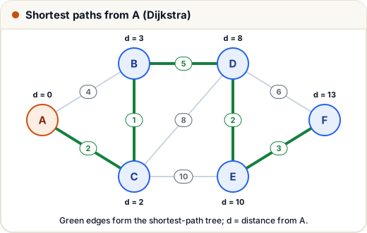
Look at B: the direct link A–B costs 4, but A–C–B costs 2 + 1 = 3. Dijkstra finds the cheaper indirect path.
import heapq

graph = {
    "A": {"B": 4, "C": 2},
    "B": {"A": 4, "C": 1, "D": 5},
    "C": {"A": 2, "B": 1, "D": 8, "E": 10},
    "D": {"B": 5, "C": 8, "E": 2, "F": 6},
    "E": {"C": 10, "D": 2, "F": 3},
    "F": {"D": 6, "E": 3},
}

def dijkstra(graph, src):
    dist = {v: float("inf") for v in graph}
    prev = {v: None for v in graph}
    dist[src] = 0
    pq = [(0, src)]
    while pq:
        d, u = heapq.heappop(pq)
        if d > dist[u]:
            continue                      # an old, longer entry
        for v, w in graph[u].items():
            if d + w < dist[v]:
                dist[v], prev[v] = d + w, u
                heapq.heappush(pq, (dist[v], v))
    return dist, prev

def path(prev, node):
    out = []
    while node:
        out.append(node)
        node = prev[node]
    return "-".join(reversed(out))

dist, prev = dijkstra(graph, "A")
for v in graph:
    print(v, dist[v], path(prev, v))
A 0 A
B 3 A-C-B
C 2 A-C
D 8 A-C-B-D
E 10 A-C-B-D-E
F 13 A-C-B-D-E-F
The routing table of A only needs the next hop: for every destination except C itself, A sends packets to C first.
OSPF (Open Shortest Path First) is the most widely used link-state protocol inside organisations. It reacts quickly to changes because every router recomputes from a complete map.
3. Distance-vector routing (Bellman-Ford)
In distance-vector routing, a router does not know the map. It knows only:
- the cost to each neighbour, and
- the distance vector each neighbour sends it — a list of "my distance to every destination".
Each router then applies the Bellman-Ford equation:
D(A, x) = min over neighbours v of [ cost(A, v) + D(v, x) ]
In words: "my distance to x is the best of (cost to reach a neighbour + that neighbour's distance to x)". It is like asking your friends how far each of them is from the railway station and adding how far you are from each friend.
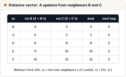
Routers exchange vectors again and again until nothing changes. The simulation below starts with each router knowing only its direct links:
graph = {
    "A": {"B": 4, "C": 2},
    "B": {"A": 4, "C": 1, "D": 5},
    "C": {"A": 2, "B": 1, "D": 8, "E": 10},
    "D": {"B": 5, "C": 8, "E": 2, "F": 6},
    "E": {"C": 10, "D": 2, "F": 3},
    "F": {"D": 6, "E": 3},
}
INF = float("inf")
# every router starts knowing only its direct links
vec = {u: {v: (0 if v == u else graph[u].get(v, INF)) for v in graph} for u in graph}

rounds = 0
while True:
    changed = False
    new = {}
    for u in graph:                   # all routers exchange at the same time
        new[u] = {}
        for x in graph:
            best = 0 if x == u else min(graph[u][v] + vec[v][x] for v in graph[u])
            new[u][x] = best
            if best != vec[u][x]:
                changed = True
    if not changed:
        break
    vec, rounds = new, rounds + 1

print("rounds with changes:", rounds)
print("A's table:", vec["A"])
rounds with changes: 4
A's table: {'A': 0, 'B': 3, 'C': 2, 'D': 8, 'E': 10, 'F': 13}
After four rounds of exchange, A's table matches Dijkstra's answer — without A ever seeing the full map.
RIP (Routing Information Protocol) is the classic distance-vector protocol. It uses hop count as the cost, sends its table every 30 seconds, and treats 16 hops as infinity — so it only suits small networks.
4. The count-to-infinity problem
Distance vector has one famous weakness: bad news travels slowly.
Take a simple chain A — B — C with every link costing 1. A reaches C through B at cost 2. Now the link B–C fails.
B has lost its direct route. But A is still advertising "I can reach C at cost 2". B does not know that A's route goes through B itself, so it believes it and sets its own distance to 1 + 2 = 3, via A. Then A updates through B, and so on:
| Exchange | A's distance to C | B's distance to C |
|---|---|---|
| before failure | 2 | 1 |
| 1 | 2 | 3 (via A) |
| 2 | 4 (via B) | 3 |
| 3 | 4 | 5 |
| 4 | 6 | 5 |
| … | keeps rising | keeps rising |
The two routers bounce packets between themselves while the numbers climb until they reach "infinity" (16 in RIP).
Fixes:
- Split horizon — never advertise a route back to the neighbour you learned it from. A would not tell B about C at all.
- Poison reverse — advertise it back, but with distance infinity: "do not use me to reach C".
- Hold-down timers — after a route goes bad, ignore new information about it for a while.
- A maximum distance (16 in RIP) — so the counting at least stops.
Split horizon fixes loops between two routers, but not every loop involving three or more routers.
5. Link state vs distance vector
| Link state | Distance vector | |
|---|---|---|
| Each router knows | the whole map | neighbours' distance vectors |
| Algorithm | Dijkstra | Bellman-Ford |
| Messages | link info, flooded to all | full table, to neighbours only |
| Convergence | fast | slow; count-to-infinity possible |
| Memory and CPU | more | less |
| Example | OSPF, IS-IS | RIP |
6. Routing across the internet: BGP
The internet is made of many independent networks called autonomous systems (AS) — for example, an internet service provider, a big company or a cloud provider. Two levels of routing exist:
- Interior gateway protocols (inside one AS): OSPF, RIP, IS-IS.
- Exterior gateway protocol (between ASes): BGP (Border Gateway Protocol).
BGP is a path-vector protocol: each route carries the full list of ASes it passes through. A router rejects a route that already contains its own AS number, which prevents loops. BGP chooses routes mainly by policy (business agreements between networks), not just the shortest path. A wrong BGP announcement can send traffic for a big website to the wrong network — such incidents have caused real outages.
Common mistakes
- Saying distance-vector routers know the full topology — they only know their neighbours' vectors.
- Picking the direct link without checking cheaper indirect paths (A–B = 4, but A–C–B = 3).
- Saying Dijkstra works with negative edge costs — it does not; Bellman-Ford handles them (link costs in networks are positive anyway).
- Thinking split horizon solves every loop — it fixes two-router loops only.
- Calling BGP a link-state protocol — it is path vector, and it runs between autonomous systems.
Quick recap
- Routers build routing tables of next hops; the best path has the lowest total cost.
- Link state: flood the map, every router runs Dijkstra (OSPF).
- Distance vector: D(A, x) = min over neighbours [cost + neighbour's distance] (RIP; 16 = infinity).
- Count-to-infinity: bad news spreads slowly; split horizon, poison reverse and hold-down timers help.
- BGP is a path-vector protocol between autonomous systems, driven by policy.