AdvancedOperating Systems · Lesson 10 of 12 · Updated ·
CPU Scheduling Numericals — Priority, HRRN, Idle CPU, Quantum Size and Context-Switch Overhead
Lesson 3 solved FCFS, SJF, SRTF and Round Robin on one simple set of processes. Exam papers add twists: priorities, a process that arrives after the CPU has gone idle, the response ratio of HRRN, and context-switch time. This lesson solves each twist with a computed Gantt chart, so you can check every number.
Reminder of the three formulas you need for every question:
| Quantity | Formula |
|---|---|
| Turnaround time (TAT) | completion time − arrival time |
| Waiting time (WT) | TAT − burst time |
| Response time (RT) | first time on the CPU − arrival time |
1. Priority scheduling — the data
Each process has a priority number. In this lesson a smaller number means a higher priority (priority 1 beats priority 3). Some books use the opposite rule, so always read the question.
| Process | Arrival | Burst | Priority |
|---|---|---|---|
| P1 | 0 | 4 | 3 |
| P2 | 1 | 3 | 1 |
| P3 | 2 | 5 | 4 |
| P4 | 4 | 2 | 2 |
| P5 | 15 | 3 | 2 |
Notice P5 arrives at 15 — later than everyone else has finished. That creates an idle gap.
2. Non-preemptive priority
Once a process starts, it runs to the end. When the CPU becomes free, pick the highest-priority process that has arrived.
- t = 0: only P1 is here → P1 runs 0–4.
- t = 4: P2 (pri 1), P3 (pri 4), P4 (pri 2) are waiting → P2 runs 4–7.
- t = 7: P4 (pri 2) beats P3 (pri 4) → P4 runs 7–9, then P3 runs 9–14.
- t = 14: nobody is ready. The CPU is idle until P5 arrives at 15. P5 runs 15–18.
| Process | CT | TAT | WT |
|---|---|---|---|
| P1 | 4 | 4 | 0 |
| P2 | 7 | 6 | 3 |
| P3 | 14 | 12 | 7 |
| P4 | 9 | 5 | 3 |
| P5 | 18 | 3 | 0 |
Average WT = (0 + 3 + 7 + 3 + 0) / 5 = 2.6. Average TAT = 30 / 5 = 6.0.
The idle gap does not count as waiting. P5 waited 0 units: it arrived at 15 and started at 15. The idle time only affects CPU utilisation: the CPU was busy 17 of 18 units = 94.4%.
3. Preemptive priority
Now a newly arrived process with a higher priority takes the CPU away immediately.
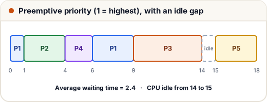
- t = 1: P2 (pri 1) arrives, beats P1 (pri 3) → P1 is preempted after 1 unit.
- t = 4: P2 finishes. P4 (pri 2) arrived at 4, and it beats P1 (3) and P3 (4) → P4 runs 4–6.
- t = 6: P1 (3 units left) beats P3 → P1 runs 6–9, then P3 9–14, idle, P5 15–18.
WT: P1 = 9 − 0 − 4 = 5, P2 = 0, P3 = 7, P4 = 0, P5 = 0 → average 2.4, average TAT 5.8.
Here is a small simulator that produces exactly these numbers. It moves the clock one unit at a time, which is the simplest way to get preemption right:
def priority_preemptive(procs):
    remaining = {name: burst for name, arr, burst, pri in procs}
    t, gantt = 0, []
    while any(remaining.values()):
        ready = [p for p in procs if p[1] <= t and remaining[p[0]] > 0]
        name = min(ready, key=lambda p: (p[3], p[1]))[0] if ready else "idle"
        if gantt and gantt[-1][0] == name:
            gantt[-1][2] = t + 1          # same process keeps running
        else:
            gantt.append([name, t, t + 1])
        if name != "idle":
            remaining[name] -= 1
        t += 1
    return gantt

procs = [("P1", 0, 4, 3), ("P2", 1, 3, 1), ("P3", 2, 5, 4), ("P4", 4, 2, 2), ("P5", 15, 3, 2)]
gantt = priority_preemptive(procs)
print(" | ".join(f"{n} {s}-{e}" for n, s, e in gantt))
finish = {n: e for n, s, e in gantt}
waits = [finish[n] - arr - burst for n, arr, burst, pri in procs]
print("waiting times:", waits, "average:", sum(waits) / len(waits))
P1 0-1 | P2 1-4 | P4 4-6 | P1 6-9 | P3 9-14 | idle 14-15 | P5 15-18
waiting times: [5, 0, 7, 0, 0] average: 2.4
Starvation. With a steady stream of high-priority jobs, a low-priority job (like P3) may wait for ever. The standard fix is aging: slowly raise the priority of a process the longer it waits.
4. HRRN — Highest Response Ratio Next
HRRN is non-preemptive. Each time the CPU becomes free, compute for every waiting process:
Response ratio = (waiting time so far + burst) / burst
and run the largest ratio. Short jobs start with a high ratio, but a long job's ratio keeps growing while it waits — so HRRN favours short jobs without starving long ones.
| Process | Arrival | Burst |
|---|---|---|
| A | 0 | 3 |
| B | 2 | 6 |
| C | 4 | 4 |
| D | 6 | 5 |
| E | 8 | 2 |
- t = 0: only A → A runs 0–3.
- t = 3: only B has arrived → B runs 3–9.
- t = 9: C = (5 + 4)/4 = 2.25, D = (3 + 5)/5 = 1.6, E = (1 + 2)/2 = 1.5 → C runs 9–13.
- t = 13: D = (7 + 5)/5 = 2.4, E = (5 + 2)/2 = 3.5 → E runs 13–15.
- t = 15: D runs 15–20.
Waiting times: A 0, B 1, C 5, D 9, E 5 → average 4.0; average TAT 8.0.
Notice step t = 9: plain SJF would have picked E (burst 2). HRRN picked C because C had already waited 5 units.
5. How the Round Robin quantum changes the answer
Take the four processes from lesson 3 (P1 0/5, P2 1/3, P3 2/8, P4 3/6) and only change the quantum:
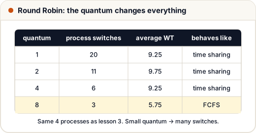
Two lessons from this table:
- A very small quantum gives fast response (everyone gets the CPU quickly) but causes many process switches — and each switch costs time.
- A quantum at least as large as the longest burst makes Round Robin identical to FCFS: nobody is ever preempted.
Average waiting time does not move smoothly with the quantum (9.25 → 9.75 → 9.25). Never assume "bigger quantum, lower waiting time" — compute it.
6. Context-switch overhead
Every switch from one process to another takes some time s during which no user work is done. If each process uses its full quantum q before switching:
CPU efficiency = q / (q + s)
| q | s | Efficiency |
|---|---|---|
| 4 ms | 1 ms | 4/5 = 80% |
| 10 ms | 1 ms | 10/11 ≈ 90.9% |
| 100 ms | 1 ms | 100/101 ≈ 99.0% |
This is why real systems use a quantum much larger than the switch time — often a few milliseconds against a switch of a few microseconds — while keeping it small enough that interactive programs feel responsive.
Worked example. Three processes with bursts 4, 3 and 5 ms arrive at time 0. FCFS, with a 1 ms context switch between processes (none before the first). Timeline: P1 0–4, switch 4–5, P2 5–8, switch 8–9, P3 9–14. All work ends at 14; useful work = 12 ms. Utilisation = 12/14 ≈ 85.7%.
Common mistakes
- Counting idle CPU time as waiting time for the next process.
- Using "larger number = higher priority" when the question says the opposite (or the other way round).
- In HRRN, using only the burst time — the ratio needs the waiting time so far, measured at the moment of the decision.
- Adding a context switch before the very first process when the question does not say so.
- Assuming a larger quantum always lowers the average waiting time.
Quick recap
- Preemptive priority: check at every arrival; a higher priority takes the CPU at once.
- An idle gap lowers CPU utilisation but adds no waiting time.
- HRRN ratio = (W + S) / S; it favours short jobs and avoids starvation.
- RR with quantum ≥ longest burst behaves like FCFS; a tiny quantum means many switches.
- Efficiency with context switches = q / (q + s).