AdvancedDiscrete Mathematics · Lesson 13 of 14 · Updated ·
Discrete Probability — Sample Spaces, Conditional Probability, Independence, Bayes' Theorem and Expected Value
Probability in a discrete maths course is counting with a fraction at the end. You already know how to count from the counting lesson. Here we turn counts into probabilities, learn how new information changes a probability (conditional probability and Bayes' theorem), and find the average outcome of a random process (expected value). These ideas are used in algorithm analysis (average-case running time, hashing, randomised quicksort) and in machine learning (naive Bayes).
We use Python's Fraction so every answer is exact, like a hand calculation, instead of a rounded decimal.
1. Sample spaces and events
- An experiment is something with an uncertain result: rolling two dice.
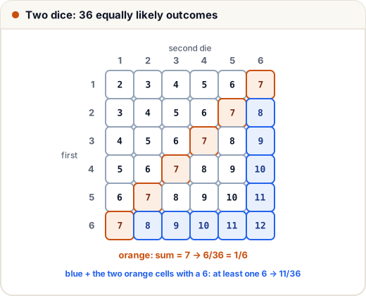
- The sample space S is the set of all possible outcomes: the 36 pairs (first die, second die).
- An event E is a subset of S: "the sum is 7".
When every outcome is equally likely:
P(E) = |E| / |S|
Three rules follow directly:
| Rule | Formula |
|---|---|
| Range | 0 ≤ P(E) ≤ 1, P(S) = 1 |
| Complement | P(not E) = 1 − P(E) |
| Union | P(E ∪ F) = P(E) + P(F) − P(E ∩ F) |
The complement rule is the most useful trick: "at least one six" is hard to count directly, but "no six" is just 5 × 5 = 25 outcomes, so P(at least one 6) = 1 − 25/36 = 11/36.
2. Conditional probability and independence
Conditional probability answers: "given that F happened, how likely is E?" We throw away every outcome outside F and count again:
P(E | F) = P(E ∩ F) / P(F) (when P(F) > 0)
Example: given that the first die is even, what is the chance the sum is 8? The first die is even in 18 outcomes; of these, (2,6), (4,4), (6,2) have sum 8. So P = 3/18 = 1/6.
Two events are independent when knowing one does not change the other:
E and F are independent ⇔ P(E ∩ F) = P(E) × P(F)
from fractions import Fraction
from itertools import product

S = list(product(range(1, 7), repeat=2))          # sample space: 36 equally likely outcomes

def P(event, given=lambda o: True):
    space = [o for o in S if given(o)]
    return Fraction(sum(1 for o in space if event(o)), len(space))

print("|S| =", len(S))
print("P(sum = 7)            =", P(lambda o: sum(o) == 7))
print("P(at least one 6)     =", P(lambda o: 6 in o))
print("P(no 6), via 1 - P    =", 1 - P(lambda o: 6 in o))
print("P(sum = 8 | first even) =", P(lambda o: sum(o) == 8, given=lambda o: o[0] % 2 == 0))

A = lambda o: o[0] % 2 == 0          # first die even
B = lambda o: sum(o) == 7            # sum is 7
C = lambda o: sum(o) == 8            # sum is 8
both = lambda e, f: (lambda o: e(o) and f(o))
print("A, B independent?", P(both(A, B)) == P(A) * P(B))
print("A, C independent?", P(both(A, C)) == P(A) * P(C), "-", P(both(A, C)), "vs", P(A) * P(C))
|S| = 36
P(sum = 7)            = 1/6
P(at least one 6)     = 11/36
P(no 6), via 1 - P    = 25/36
P(sum = 8 | first even) = 1/6
A, B independent? True
A, C independent? False - 1/12 vs 5/72
The result surprises many students. "Sum is 7" is independent of "first die is even": whatever the first die shows, exactly one value of the second die makes 7. "Sum is 8" is not independent of it: if the first die is 1, a sum of 8 is impossible. Never guess independence; check the formula.
Do not confuse independent with mutually exclusive (P(E ∩ F) = 0). Two mutually exclusive events with non-zero probabilities are never independent: if one happens, the other certainly did not.
3. Total probability and Bayes' theorem
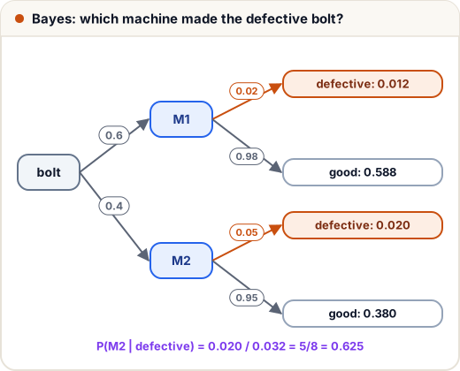
A factory has two machines. In this example, M1 makes 60% of the bolts and 2% of its bolts are defective; M2 makes 40% and 5% of its bolts are defective. (These numbers are chosen for the example.)
Law of total probability. Split by which machine made the bolt:
P(D) = P(M1)·P(D | M1) + P(M2)·P(D | M2) = 0.6 × 0.02 + 0.4 × 0.05 = 0.012 + 0.020 = 0.032
Bayes' theorem turns the condition around. We picked a defective bolt. Which machine probably made it?
P(M2 | D) = P(M2)·P(D | M2) / P(D) = 0.020 / 0.032 = 5/8
from fractions import Fraction as F

# a factory: machine M1 makes 60% of the bolts, M2 makes 40%
prior = {"M1": F(60, 100), "M2": F(40, 100)}
defect_rate = {"M1": F(2, 100), "M2": F(5, 100)}

# total probability: P(D) = sum over machines of P(M) * P(D | M)
p_d = sum(prior[m] * defect_rate[m] for m in prior)
print("P(defective) =", p_d, "=", float(p_d))

# Bayes: P(M | D) = P(M) * P(D | M) / P(D)
for m in prior:
    post = prior[m] * defect_rate[m] / p_d
    print(f"P({m} | defective) = {post} = {float(post):.4f}")
P(defective) = 4/125 = 0.032
P(M1 | defective) = 3/8 = 0.3750
P(M2 | defective) = 5/8 = 0.6250
M2 makes fewer bolts, but because its defect rate is higher it is responsible for most defective ones. The two posterior probabilities add up to 1, which is a quick check on your arithmetic.
4. Random variables and expected value
A random variable X gives a number to each outcome, like "the sum of the two dice". Its expected value is the probability-weighted average:
E[X] = Σ x · P(X = x)
The most useful fact is linearity of expectation: E[X + Y] = E[X] + E[Y], always, even when X and Y are not independent. That lets you split a hard average into easy pieces.
The binomial formula counts successes in n independent trials, each with success probability p:
P(exactly k successes) = C(n, k) · pᵏ · (1 − p)ⁿ⁻ᵏ
from fractions import Fraction as F
from itertools import permutations, product
from math import comb

die = range(1, 7)
E_die = sum(F(x, 6) for x in die)
E_two = sum(F(a + b, 36) for a, b in product(die, repeat=2))
print("E[one die] =", E_die, "  E[sum of two dice] =", E_two, "= 2 * E[one die]?", E_two == 2 * E_die)

# binomial: exactly k heads in n fair coin tosses
n = 5
for k in range(n + 1):
    print(f"P({k} heads in {n}) = {comb(n, k)}/{2 ** n}")

# expected number of people who get their own hat back (fixed points of a random permutation)
for n in [3, 4, 5]:
    perms = list(permutations(range(n)))
    fixed = sum(sum(p[i] == i for i in range(n)) for p in perms)
    print(f"n = {n}: average fixed points = {F(fixed, len(perms))}")
E[one die] = 7/2   E[sum of two dice] = 7 = 2 * E[one die]? True
P(0 heads in 5) = 1/32
P(1 heads in 5) = 5/32
P(2 heads in 5) = 10/32
P(3 heads in 5) = 10/32
P(4 heads in 5) = 5/32
P(5 heads in 5) = 1/32
n = 3: average fixed points = 1
n = 4: average fixed points = 1
n = 5: average fixed points = 1
The last result is a classic. n people throw their hats in a pile and each picks one at random. How many, on average, get their own hat back? Let Xᵢ = 1 if person i gets their own hat. Each person does so with probability 1/n, so E[Xᵢ] = 1/n. By linearity, the expected total is n × 1/n = 1, for every n. The Xᵢ are not independent, but linearity does not care. (The derangements count the opposite case: nobody gets their own hat.)
Common mistakes
- Using |E| / |S| when outcomes are not equally likely. For the sum of two dice, the 11 possible sums (2 to 12) are not equally likely; count the 36 pairs instead.
- Adding probabilities of overlapping events without subtracting P(E ∩ F).
- Mixing up P(E | F) and P(F | E). P(defective | M2) = 0.05, but P(M2 | defective) = 5/8. Bayes' theorem converts one into the other.
- Treating "mutually exclusive" as "independent". They are almost opposites.
- Believing linearity of expectation needs independence. It does not; only E[XY] = E[X]E[Y] needs independence.
Quick recap
- Equally likely outcomes: P(E) = |E| / |S|. Complement: 1 − P(E).
- P(E | F) = P(E ∩ F) / P(F). Independent ⇔ P(E ∩ F) = P(E)P(F).
- Total probability: P(D) = Σ P(Mᵢ) P(D | Mᵢ). Bayes: P(Mᵢ | D) = P(Mᵢ) P(D | Mᵢ) / P(D).
- E[X] = Σ x P(X = x); E[X + Y] = E[X] + E[Y] always.
- Binomial: C(n, k) pᵏ (1 − p)ⁿ⁻ᵏ.